Trade and Technology Adoption in Distorted Economies
Farid Farrokhi (Purdue University)
Ahmad Lashkaripour (Indiana University, CESifo, CEPR)
Heitor S. Pellegrina (University of Notre Dame)
Journal of International Economics · July 2024
Read PDF · Markdown source · Reader view
Abstract. This paper examines how labor market imperfections distort firm-level technology choices and alter the gains from trade in developing countries. Motivated by evidence that firms using modern technologies are disproportionately exposed to labor market distortions, we introduce firm-level technology choices and labor market distortions into an otherwise standard quantitative trade model. We then provide formulas for the welfare and labor productivity gains from trade liberalization, highlighting the role of distortions and technology choice. Our quantitative analysis reveals that labor market distortions provide a possible explanation for the inefficiently low levels of modern technology adoption in developing countries. Moreover, labor market distortions erode one-third of the potential labor productivity gains from trade liberalization among low-income countries.
1 Introduction
In the past four decades, developing countries have become significantly more integrated into global supply chains. This process has spurred the emergence of modern manufacturing firms operating with advanced technologies that make intensive use of internationally-sourced intermediate inputs.
Yet, it remains a matter of debate whether the integration of developing countries into the world trade system has delivered the expected dividends. The critics of this process emphasize two apparent anomalies. First, the rate of modern technology adoption in many low-income countries remains unusually low despite recent episodes of trade liberalization (Hsieh and Klenow, 2014; Buera et al., 2021). Second, the adoption of modern technologies in some developing countries has coincided with a stagnation of aggregate labor productivity (Diao et al., 2021).
The existing literature provides a few possible explanations for these so-called anomalies. The big-push theories of economic development identify fixed production costs and inadequate market size as the main barriers to modern technology adoption in low-income countries (Murphy et al., 1989). Another body of literature on (in)appropriate technologies attributes the above patterns to a possible mismatch between modern technologies and the resource endowment of low-income countries (Basu and Weil, 1998; Acemoglu and Zilibotti, 2001).
Appealing to economic theory and detailed firm-level data, we argue that labor market distortions provide another explanation for these two anomalies. We, specifically, introduce two key ingredients into an otherwise standard quantitative trade model: technology adoption and labor market distortions. We demonstrate analytically how these two ingredients interact in open economies, shaping aggregate labor productivity and welfare. Moreover, we quantify our model and show that labor market distortions lead to inefficiently low adoption of modern technologies and curtail the impacts of trade-led modern manufacturing growth on aggregate labor productivity in low-income countries.
The model we develop is a multi-country, multi-industry general equilibrium framework in which firms self-select into traditional or modern technology types in the presence of labor market distortions. Each country, in addition to its labor force, is endowed with a continuum of heterogenous firms, each corresponding to a unit of managerial capital. Firms in each industry select the technology type that maximizes their profits. Technologies differ in their total factor productivity and the intensity by which they use managerial capital, labor, and intermediate inputs. In the empirically relevant case, modern technologies are labor-saving and intermediate-input intensive. Consequently, a reduction in trade barriers that provides cheaper access to foreign intermediate inputs raises relative returns to modern technologies. This development incentivizes the adoption of modern technologies, the rate of which is regulated by a “technology elasticity,” à la Farrokhi and Pellegrina (2023). Labor market distortions, meanwhile, vary across countries and across firm types within each country. We model these distortions as labor market wedges that create a gap between the cost of labor to firms and the actual payment to workers.
We begin our theoretical analysis by deriving three formulas to dissect the mechanisms that shape welfare (defined as aggregate real consumption). First, we show that (in a stylized closed economy version of our model) the welfare cost of misallocation depends on the cross-technology dispersion in labor wedges. Second, we decompose the first-order welfare effects of trade liberalization (i.e., trade cost reductions) into three components: (i) the well-known ACR component (Arkolakis et al., 2012), (ii) the change to allocative efficiency, and (iii) residual terms of trade and technology selection effects.These residual terms reflect our model’s accommodation of managerial capital (a quasi-fixed input) and endogenous technology choice, both of which are absent in the baseline ACR framework. Our welfare accounting formulas are related to Baqaee and Farhi (2019) and Atkin and Donaldson (2021), but are structured differently to emphasize our connection to the canonical ACR formula. Third, we derive a formula for the welfare gains from trade relative to autarky.
Additionally, we show that aggregate labor productivity (defined as the economy-wide gross output per worker) can be expressed as the national-level real wage adjusted for trade openness and labor allocation across industries and technology types. We then derive a formula that characterizes the first-order impact of trade liberalization on aggregate labor productivity. This formula incorporates similar mechanisms that shape welfare but, importantly, highlights the differential effects of trade on aggregate labor productivity and welfare.
Having established these analytical results, we take our model to data on 99 countries (plus a rest of the world aggregate). To this end, we use country-level input-output data from the Global Trade Analysis Project (GTAP). We combine these country-level data with technology-type-level statistics that we construct using firm-level data from the World Bank Enterprise Survey (hereafter, WBES), which is available for a large set of countries at different levels of development. These statistics include estimated labor intensities, labor market wedges, and the share of firms in modern and traditional technologies across countries. We simulate our model using the exact hat algebra method, sidestepping the need to calibrate productivity shifters and trade costs.
We start our quantitative analysis by decomposing the welfare impacts of trade liberalization for each economy. We find that the non-ACR channels—i.e., improvements to allocative efficiency and residual terms of trade—make a positive contribution across all country groups, raising the gains from trade liberalization in our framework relative to ACR. The contribution from these non-ACR channels is about two times larger among low-income countries relative to high-income counterparts, with the allocative efficiency channel being the major contributor. Intuitively, trade liberalization encourages modern technology adoption and directs factors of production toward modern technologies, both of which improve allocative efficiency, since modern firms are exposed to larger distortions. These allocative efficiency gains are more pronounced among low-income countries, which suffer from initially-higher levels of misallocation.
Lastly, we tackle the primary question that has motivated our research: How do labor market distortions modify the labor productivity gains from trade liberalization among developing countries? To provide an answer, we design an experiment to evaluate how labor market distortions, and their interaction with technology adoption, alter the aggregate labor productivity gains from trade. We consider a twenty percent reduction in trade costs facing low-income countries and compare the impacts of this trade cost shock in economies with and without labor market distortions. Our results reveal that the interplay between trade liberalization and labor market distortions is crucial: Among low-income countries, labor market distortions erode (on average) one-third of the potential labor productivity gains from trade liberalization. Intuitively, trade liberalization raises aggregate labor productivity by improving access to imported intermediate inputs and directing resources towards modern technologies that rely more intensively on intermediate inputs. In distorted economies, however, the productivity gains from trade liberalization are hampered by the fact that modern technologies are disproportionately-exposed to labor market wedges.We notice that labor market distortions can amplify the welfare gains from trade (i.e., aggregate real consumption), but still attenuate the aggregate labor productivity gains from trade (i.e., gross output per worker). The two outcomes can diverge in open economies that utilize intermediate inputs, depending on the underlying changes to the terms of trade and aggregate value added shares. We elaborate further on this point in Section 3.4.
In what follows, we first outline our contribution to the literature. Section 2 then provides motivating evidence for our framework, using previously-documented facts from the literature and our own estimates of labor distortions based on the WBES. Section 3 lays out our theoretical model. Section 4 presents analytical results from the model. Section 5 describes the calibration of the model. Section 6 presents our quantitative results. Section 7 discusses alternative calibrations approaches and the robustness of our baseline model. Section 8 concludes.
This paper contributes to research evaluating how misallocation interacts with international trade, including studies on the role of firm-level distortions (Bai et al., 2019; Scottini, 2018; Ding et al., 2023), the impact of distortions on the world’s input-output structure (Caliendo et al., 2017), the decomposition of the welfare gains from trade shocks (Baqaee and Farhi, 2019), and the interactions of distortions with trade policy (Lashkaripour and Lugovskyy, 2023; Bartelme et al., 2019)—see Atkin and Donaldson (2021) and Atkin and Khandelwal (2020) for reviews of recent research.See Hsieh and Klenow (2009) for seminal work on the impact of misallocation on aggregate output. Relative to this literature, we examine the effects of factor market distortions on firms’ technology choice, where technologies differ in their factor intensity. We find that labor market distortions can substantially reduce the productivity gains from trade liberalization in low-income countries.
By studying the role of technology choices, our paper speaks to research on technology adoption. Closer to our work, this front of research has examined the interactions between trade and technology upgrading (Yeaple, 2005; Bustos, 2011; Davidson et al., 2008), finance and misallocation (Midrigan and Xu, 2014), economic shocks and capital intensity (Oberfield, 2013), and technology adoption in developing economics (Verhoogen, 2021).There is also a rich literature analyzing the effects of trade on firms’ technology choices in developing economies, see De Loecker et al. (2016) and Goldberg et al. (2010) for India, Bustos (2011) for Argentina,Medina (2020) for Peru, Pavcnik (2017) and Oberfield (2013) for Chile, and Fieler et al. (2018) for Colombia. We complement these studies by examining the interaction between technology adoption and technology-specific misallocation. To the best of our knowledge, we are the first to study technology choices in open economies with distorted labor markets. In our analysis, labor market distortions lead to distorted technology choices—specifically, firms’ adoption of modern technologies is low relative to an efficient economy.
More broadly, this paper contributes to a large literature that formulates quantitative equilibrium models to evaluate the welfare gains from trade, following the seminal work of Eaton and Kortum (2002) and the research reviewed by Costinot and Rodríguez-Clare (2014). In the past two decades, this literature has developed an abundance of new tools and significantly expanded its scope of analysis, covering topics such as workers’ mobility (Caliendo et al., 2019; Artuç et al., 2010), input-output structures of trade (Caliendo et al., 2017), agricultural trade (Sotelo, 2020; Farrokhi and Pellegrina, 2023), scale economies (Kucheryavyy et al., 2023; Lashkaripour and Lugovskyy, 2023; Farrokhi and Soderbery, 2023; Bartelme et al., 2019), non-homothetic preferences (Fieler, 2011), multinational firms (Ramondo and Rodríguez-Clare, 2013), among many others. Our contribution to this broader literature is to endogenize technology choices in manufacturing and examine its interactions with domestic market distortions. 2
2 Motivating Evidence
This section draws upon existing literature to motivate the building blocks of our model. We examine the interplay between technology adoption, firm size, and distortions in previous studies. Additionally, we present preliminary data patterns from the WBES data that align with the motivating factors we document, and which will later inform the calibration of our model.
Firm Size, Technology and Distortions. Our theoretical framework builds on a well-established finding in the literature: larger firms tend to have higher capital requirements and be more intensive in intermediate inputs. This observation has motivated the formulation of several theoretical frameworks to study the interactions between technology and input distortions, including Ciccone (2002) and Acemoglu et al. (2007). Notably, using firm-level data, Midrigan and Xu (2014), Lagakos (2016) and Buera et al. (2021) have quantified models in which larger, modern firms tend to be more intermediate input-intensive (or more capital-intensive) compared to smaller, traditional firms. In particular, a growing number of quantitative papers find that input distortions can have substantial aggregate implications to productivity.See, for example, Lanteri et al. (2023), Morlacco (2019), and Zavala (2022). These papers have focused on different types of input distortions: Lanteri et al. (2023) focuses on capital, Morlacco (2019) on intermediate inputs, and Zavala (2022) on farmers’ output as an input to traders.
Labor Market Distortions. Our framework will incorporate the impact of distortionary regulations and taxes on labor, which are prevalent in many developing countries. Atkin and Khandelwal (2020) and Atkin and Donaldson (2021) provide a comprehensive review of the literature on trade and distortions. Studies such as Hopenhayn and Rogerson (1993), Besley and Burgess (2004), and Haltiwanger et al. (2014) have shown large aggregate productivity effects of laws that facilitate the relocation of firms within the economy. Importantly, many of these regulations disproportionately burden larger firms, as evidenced from research on India by Bertrand et al. (2021) and on Brazil by Ulyssea (2018). To avoid these regulations and taxes, firms remain small and operate in the informal sector. These regulations have been shown to have significant negative effects on the economy (Meghir et al., 2015; Ulyssea, 2018; Dix-Carneiro et al., 2021). In particular, Ulyssea (2018) identifies empirical regularities linking firm size and formality, and finds that larger firms tend to employ a smaller proportion of informal workers.Additionally, Hsieh and Klenow (2014) show systematic size differences between firms in formal and informal sectors for India and Mexico. In line with these findings from the literature, Appendix Table A.2 (column 3) shows that larger firms tend to face larger labor market regulations in the WBES data, particularly in less-developed countries.
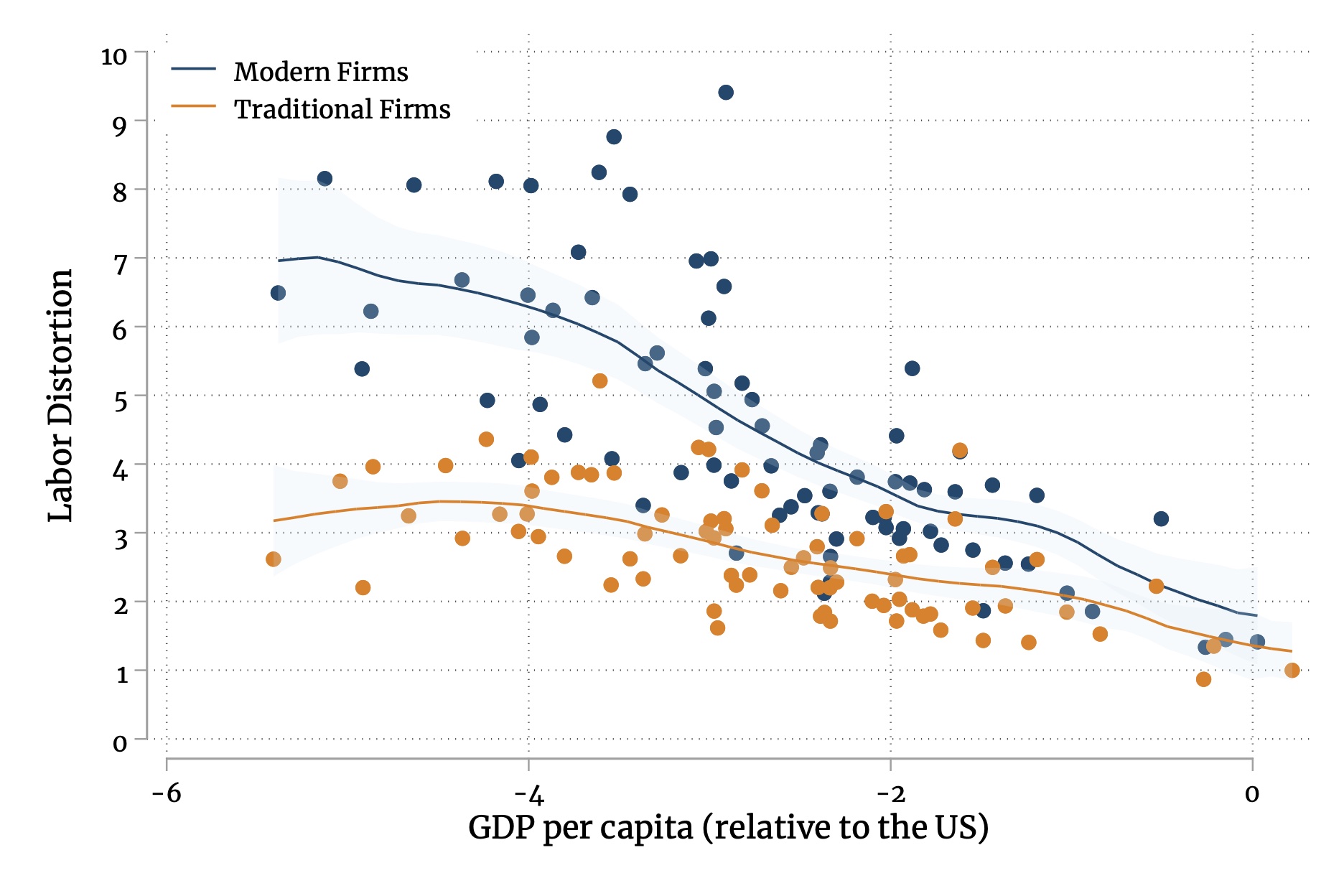 Notes: This figure shows the distribution of labor wedges across countries at different levels of economic
development. Modern and traditional firms are classified based on their size. Section 6 describes the procedure that
we use to recover such labor wedges.
Notes: This figure shows the distribution of labor wedges across countries at different levels of economic
development. Modern and traditional firms are classified based on their size. Section 6 describes the procedure that
we use to recover such labor wedges.Labor Market Distortions and Firm Size in the WBES. To close this section, we provide a first look at the firm-level data from the WBES and show how it speaks to the above-mentioned empirical patterns from the literature. Figure 1 reports our estimates of the labor wedge for modern and traditional firms (classified based on their size) across countries in different levels of development—later, in Section 5, we describe our classification and estimation procedure. Labor distortions are generally higher in less developed countries, and particularly so for modern firms.
Motivated by these aforementioned patterns, our model introduces the notion that labor wedges can vary by a country’s level of economic development and by the type of technology—traditional (labor-intensive) versus modern (intermediate-input-intensive). These differences, in turn, affect firms’ technology choices, and, consequently, the aggregate exposure of an economy to labor market distortions will depend on the equilibrium mix of traditional and modern firms.
3 The Model
Environment. The global economy consists of multiple countries indexed by \(i,\:j\in \mathbb {I}\) and multiple industries indexed by \(s,k\in \mathbb {\mathbb {S}}\). Production in country \(i-\) industry \(s\) can take place under two types of technology indexed by \(t\in \mathbb {T\equiv }\{0,1\}\); namely, “traditional” (\(t=0\)) and “modern” (\(t=1\)). Country \(i\) is endowed with \(\bar {L}_{i}\) units of labor and is populated by a fixed, exogenously given continuum of firms in each industry, indexed by \(\omega \in \Omega _{i,s}\). Each firm is endowed by one unit of managerial capital. Markets are perfectly competitive.
Labor Market Wedges. Each economy is subject to wedges in the labor market \(\tau _{i,st}^{L}\), which can vary not only across countries and industries, but also between modern and traditional technologies. These wedges denote the difference between the amount a firm pays to employ a worker and the amount the worker receives.
3.1 Production
The production function for firm \(\omega \in \Omega _{i,s}\) under technology \(t\) is given by:
where \(A_{i,st}\) is total factor productivity under technology \(t\), \(\mathscr {K}_{i,st}\left (\omega \right )\) is managerial capital, \(Z_{i,st}(\omega )\) is the idiosyncratic managerial productivity, \(L_{i,st}(\omega )\) is labor employment, and \(M_{i,st}(\omega )\) is a composite intermediate input. Specifically, \(M_{i,st}(\omega )=\prod _{s'\in \mathbb {S}}M_{i,ss't}(\omega )^{\phi _{i,ss't}},\) where \(M_{i,ss't}(\omega )\) is the bundle of intermediate goods that industry \(s\) purchases from industry \(s'\) (that itself aggregates over inputs sourced from various origin countries), and \(\phi _{i,ss'}\) denotes the share corresponding to origin industry \(s'\) and destination industry \(s\), with \(\sum _{s'}\phi _{i,ss'}=1\). Factor shares are given by \(\gamma _{st}^{Z},\gamma _{st}^{L},\) and \(\gamma _{st}^{M}\) and satisfy \(\gamma _{st}^{Z}+\gamma _{st}^{L}+\gamma _{st}^{M}=1\). In particular, \(\gamma _{st}^{Z}\) controls the share of payments to the managerial capital, \(\mathscr {K}_{i,st}(\omega )\), that corresponds to the share of firm’s profits, akin to Lucas (1978).Our specification is equivalent to one in which a “firm” corresponds to a manager who employs labor and intermediate inputs under a decreasing-returns-to-scale production technology. Under this terminology, returns to the managerial capital should be interpreted as the firm’s profits.
Firms’ Choices of Technology. Traditional (\(t=0\)) and modern technologies (\(t=1\)) differ in their input intensity parameters, \(\boldsymbol {\gamma }_{0}\equiv \{\gamma _{s0}^{Z},\gamma _{s0}^{L},\gamma _{s0}^{M}\}_{s}\) versus \(\boldsymbol {\gamma }_{1}\equiv \{\gamma _{s1}^{Z},\gamma _{s1}^{L},\gamma _{s1}^{M}\}_{s}\), and total factor productivity levels, \(A_{i,s0}\) versus \(A_{i,s1}\). Each firm \(\omega \in \Omega _{i,s}\) draws a vector of managerial productivity levels, \([Z_{i,s0}(\omega ),Z_{i,s1}(\omega )]\), and chooses a technology type. Per cost minimization, the marginal cost of production for a firm \(\omega \in \Omega _{i,s}\) using technology \(t\) is:
where \(r_{i,st}\left (\omega \right )\) is the return to managerial capital, \(\tau _{i,st}^{L}w_{i}\) the wage rate in country \(i\) inclusive of labor market wedges, and \(m_{i,st}\) the price of the intermediate input bundle. All firms within a country-industry, regardless of their technology type, supply the same product. Let \(p_{i,s}\) denote the competitive price supplied by country \(i-\) industry \(s\). Perfect competition ensures that \(p_{i,s}=c_{i,st}(\omega )\), which pins down firm \(\omega\)’s profits (as the return to its managerial capital) when using technology \(t\):
The firm’s profits, \(r_{i,st}(\omega )\), depends on output price, \(p_{i,s}\), the technology-specific impact from input prices,
the effective labor market wedge, \(\grave {\tau }_{i,st}^{L}\equiv \left (\tau _{i,st}^{L}\right )^{\gamma _{st}^{L}/\gamma _{st}^{Z}}\), the impact of technology-specific productivity, \(a_{i,st}\equiv \left (A_{i,st}\right )^{1/\gamma _{st}^{Z}}\), and the firm-level productivity draw, \(Z_{i,st}(\omega )\).To provide intuition for how these relative input prices matter, consider the empirically-relevant case in which the traditional technology is intensive in the use of labor, and the modern technology is intensive in the use of intermediate inputs. In that case, within each industry the return to the traditional technology falls when the relative wage \(\left (w_{i}/p_{i,s}\right )\) increases, and the return to the modern technology rises if the relative intermediate input price \(\left (m_{i,st}/p_{i,s}\right )\) decreases.
Firm \(\omega\) faces a discrete choice problem wherein it chooses technology \(t\in \mathbb {T}\) that maximizes its profits, \(r_{i,st}\left (\omega \right )\). Namely,
The vector of firm-level productivities, \(\mathbf {Z}_{i,st}(\omega )\equiv \left [Z_{i,st}(\omega )\quad for t\in \mathbb {T}\right ]\), is drawn independently by firms from a Fret distribution, \(\Pr \left (\mathbf {Z}_{i,st}(\omega )\leq \mathbf {z}_{i,st}\right )=\exp \left (-\bar {\phi }\sum _{t\in \mathbb {T}}z_{i,st}^{-\theta }\right )\), where \(\bar {\phi }\equiv \left [\Gamma \left (1-1/\theta \right )\right ]^{-\theta }\) is a normalization which ensures that \(\mathbb {E}\left [Z_{i,st}(\omega )\right ]=1\), with \(\theta >1\) governing the dispersion in productivity draws. Under this distributional assumption, the share of firms that select technology \(t\) in country \(i-\) industry \(s\), denoted by \(\alpha _{i,st}\), is:
where \(H_{i,s}\) is the industry-level average profits (relative to the output price). Intuitively, a greater share of firms select technology \(t\) if it exhibits \((i)\) a higher average productivity, \(a_{i,st}\); \((ii)\) more favorable impact from wages and intermediate input prices, as summarized by \(h_{i,st}\); and, \((iii)\) lower exposure to labor market distortions, \(\grave {\tau }_{i,st}^{L}\). The extent of these relationships is controlled by parameter \(\theta\), which we call the “technology elasticity.”
Industry Aggregates. We can now specify aggregate sales in country \(i\)–industry \(s\) given firms’ choices of technology. Let \(R_{i,st}\left (\omega \right )\equiv p_{i,s}Q_{i,st}\left (\omega \right )\) be the sales of firm \(\omega \in \Omega _{i,st}\) where \(\Omega _{i,st}\) is the set of firms in country \(i-\) industry \(s\) that choose technology \(t\); and by aggregation, \(R_{i,st}=\mathbb {E}\left [R_{i,st}(\omega )\:|\:\omega \in \Omega _{i,st}\right ]\times |\Omega _{i,s}|\). Recall that the firm’s profits is \(r_{i,st}\left (\omega \right )=Z_{i,st}(\omega )\times \left (a_{i,st}p_{i,s}h_{i,st}/\grave {\tau }_{i,st}^{L}\right )\). Since \(r_{i,st}(\omega )\) is a fraction \(\gamma _{st}^{Z}\) of firm \(\omega\)’s sales, i.e., \(R_{i,st}\left (\omega \right )=\left (\gamma _{st}^{Z}\right )^{-1}r_{i,st}\left (\omega \right )\), the value of sales in country \(i-\) industry \(s-\) technology \(t\), \(R_{i,st}\), equals:
Since the expected value of productivity draws conditional on firms’ selections equals
by normalizing \(|\Omega _{i,s}|=1\) (without of loss of generality), we can derive \(R_{i,st}\), as:
Using Equation (), the industry-level sales, \(R_{i,s}=\sum _{t\in \mathbb {T}}R_{i,st}\), can be expressed as:
where \(\alpha _{i,st}\) and \(H_{i,s}\) are given by Equation (1).
3.2 Trade and Consumption
The representative consumer in each country \(j\) receives utility \(C_{j}\) according to a two-tier preference system:
In the upper tier, the final consumption, \(C_{j}\), is a Cobb-Douglas aggregation over industry-level bundles, \(\{C_{j,s}\}_{s\in \mathbb {S}}\), with constant expenditure shares \(\beta _{j,s}\). In the lower tier, \(C_{j,s}\) is a CES aggregation over within-industry varieties that are differentiated by their origin country, \(\{C_{ij,s}\}_{i\in \mathbb {I}}\), where \(b_{ij,s}\) is a demand shifter and \(\sigma _{s}\) is the elasticity of substitution between varieties within industry \(s\).
Country \(i\)’s variety of industry \(s\) can be delivered to country \(j\) at price \(d_{ij,s}p_{i,s}\), where \(p_{i,s}\) is the producer price and \(d_{ij,s}\) is the iceberg trade costs.As is standard in the literature, we assume that \(d_{ii,s}=1\) and \(d_{ij^{\prime },s}d_{j^{\prime }j,s}>d_{ij,s}\). We assume that final consumption and intermediate input demand are characterized by the same CES function, as given by \(C_{j,s}\). Accordingly, country \(j\)’s share of expenditure on goods originating from country \(i\) within industry \(s\) is:
where \(P_{j,s}\) denotes the CES price index of industry \(s\) in location \(j\). 3.3
3.3 General Equilibrium
Market Clearing and Equilibrium. The labor market in each country \(i\) clears by ensuring that:
For each dollar that is paid to employ workers, only a fraction \(1/\tau _{i,st}\) is the payment to workers, and the remainder, \(\left (\tau _{i,st}-1\right )/\tau _{i,st}\), is the payment associated with labor wedges. Hence, all else equal, higher labor wedges lower the demand for workers. In turn, labor wedge payments amount to:
The labor wedge represents a range of costs that firms incur due to labor market distortions, e.g., bribery, theft, bureaucratic berries, labor market regulations, and search frictions. Our model takes \(\tau _{i,st}\) as a reduced-form representation of these distortions without taking a stance on their specific nature.To simplify our analysis and focus on the role of technology choices and distortions, we adopt the more common approach in which wedges are exogenous. We leave an analysis of endogenous wedges to future research.
The goods market for each country \(i-\) industry \(s\) clears by ensuring that:
where country \(i\)’s gross expenditure on industry \(s\), \(E_{i,s}\), is the sum of final good and intermediate input expenditure:
Lastly, \(Y_{i}\) denotes national income or GDP, and is given by
where \(\Pi _{i}\equiv \sum _{s\in \mathbb {S}}\sum _{t\in \mathbb {T}}\gamma _{st}^{Z}R_{i,st}\) is the aggregate profits. The above equations ensure that trade is balanced and the national expenditure net of labor-wedge payments, \(E_{i}-T_{i}\), equals the sum of factor rewards (labor wages and firms’ profits).
In what follows, we refer to \(w_{i}L_{i}/P_{i}\) as workers’ real wages and we call real national income,
as country \(i\)’s welfare, which in turn corresponds to aggregate real consumption. 3.4
3.4 Aggregate Labor Productivity (ALP)
We define aggregate labor productivity (ALP) in a country-industry pair as output per worker there—later we show quantitative results for alternative measures of ALP. Appendix A.2 shows that:
To see the intuition behind Equation (10), consider the case of one-sector efficient economy in which labor is the only factor of production.This special case corresponds to: \(L_{i,st}\equiv L_{i,t}\), \(L_{i,s}\equiv L_{i},\) \(p_{i,s}\equiv p_{i}\), \(\tau _{i,st}\equiv \tau _{i,t}=1\), and \(\gamma _{st}^{L}\equiv \gamma _{t}^{L}=1.\) In that special case, the aggregate labor productivity collapses to the ratio of wage to producer-price (\(w_{i}/p_{i}\)). In the general case, however, labor market distortions and non-labor factors enter the equation through \(\tau _{i,st}^{L}\) and \(\gamma _{st}^{L}\). In addition, one needs to take a stance on how to aggregate industry-level quantities to a national index of labor productivity. Under the assumption that industry-level output quantities are aggregated using the final consumption aggregator, i.e., \(Q_{i}=\prod _{s}\left (Q_{i,s}\right )^{\beta _{i,s}}\), the national-level ALP equals:
where \(\ell _{i,st}\equiv L_{i,st}/L_{i}\) is the share of workers in industry \(s-\) technology \(t\). In words, aggregate labor productivity, \(\text{ALP}_{i}\), equals real wage (\(w_{i}/P_{i}\)) adjusted for: (i) trade openness captured by non-unity domestic expenditure shares (second bracket), and (ii) allocation of workers across industries and technology types (third bracket). Intuitively, trade openness alters the relationship between the aggregate produce price (\(\prod _{s}p_{i,s}^{\beta _{i,s}}\)) and the final consumer price (\(P_{i}=\prod _{s}P_{i,s}^{\beta _{i,s}}\)); and, the labor allocation governs the contribution from each industry-technology pair to the aggregate labor productivity.
\(ALP\) vs. Welfare. Our objective is to explore the effects of trade on aggregate labor productivity \(\text{ALP}_{i}\) given by Equation () and welfare \(W_{i}\) by Equation (9). Linking these two measures of economic performance can, thus, provide better insight into subsequent results. As shown in Appendix A.2, \(\text{ALP}_{i}\) relates to welfare per worker \(\left (W_{i}/L_{i}\right )\) according to:
where \(y_{i,s}\equiv Y_{i,s}/Y_{i}\) is the value added share of industry \(s\) in country \(i\) and \(\bar {\gamma }_{i,s}^{M}\) is the average cost share of intermediate inputs. Two channels of effect are responsible for the difference between aggregate labor productivity and welfare. To see them most clearly, consider a single-industry version of our setup with one technology type, where the above formula simplifies to:
In a closed economy without intermediate input use, aggregate labor productivity, \(\text{ALP}_{i}\), aligns with welfare per worker, \(W_{i}/L_{i}\). Otherwise, these metrics may diverge based on the terms of trade (represented by \(\pi _{ii}^{\frac {1}{1-\sigma }}\))Note that \(\pi _{ii}^{\frac {1}{1-\sigma }}=p_{i}/P_{i}\) captures the terms of trade as the ratio of export price, governed by producer price \(p_{i}\), to import price index, \(P_{i}\). and the share of value added in gross output (\(1-\bar {\gamma }_{i}^{M}\)). From this equation, it is evident that welfare and aggregate labor productivity may react differently to an external event like trade liberalization in our model, depending on the underlying changes to the terms of trade and the aggregate value added share. 3.5
3.5 Counterfactual Analysis
Our framework is adept to study the welfare impacts of changes in trade costs and labor market wedges.In this section, we adopt the hat notation: For any generic variable \(x\) in the baseline equilibrium, let \(x^{\prime }\) be its corresponding value in the counterfactual equilibrium, and \(\hat {x}\equiv x^{\prime }/x\) denote its change from the baseline to the counterfactual equilibrium. Specifically, the sufficient statistics for counterfactual analyses in our model can be summarized by \(\mathscr {B}\equiv \{\mathscr {B}^{\text{Param}},\mathscr {B}^{\text{Data}}\}\) where \(\mathscr {B}^{\text{Param}}\equiv \{\sigma,\theta,\gamma _{st}^{L},\gamma _{st}^{M},\gamma _{st}^{Z},\tau _{i,st}^{L},\phi _{i,sk},\beta _{i,s}\}\) and \(\mathscr {B}^{\text{Data}}\equiv \{\pi _{ij,s},\alpha _{i,st},w_{i}L_{i},R_{i,st},E_{i,s},Y_{i}\}\). Given \(\mathscr {B}\), for any set of exogenous shocks to trade costs and labor wedges \(\mathscr {P}\equiv \{\hat {d}_{ij,s},\hat {\tau }_{i,st}^{L}\}\), Appendix B describes our model equilibrium in changes to trade, employment and technology shares, aggregate sales and expenditures, and prices and wages, \(\mathscr {E}\equiv \{\hat {\pi }_{ij,s},\) \(\hat {\ell }_{i,st},\) \(\hat {\alpha }_{i,st},\) \(\hat {R}_{i,st}\) \(,\hat {E}_{i,s}\) \(,\hat {Y}_{i}\) \(,\hat {P}_{i,s}\) \(,\hat {p}_{i,s}\) \(,\hat {w}_{i}\}\). Moreover, Appendix D derives the change to welfare, real wage, and aggregate labor productivity as a function of the above sufficient statistics and general equilibrium changes to domestic expenditure shares (\(\hat {\pi }_{ii,s}\)), employment shares (\(\hat {\ell }_{i,st}\)), and technology shares (\(\hat {\alpha }_{i,st}\)). 4
4 Misallocation and the Gains from Trade
This section explores the impacts of labor market distortions on the gains from trade, emphasizing the role of technology adoption. To set the stage for an open-economy analysis, we first characterize the cost of misallocation in closed economy. We then return to our general open economy setup to characterize the effects of trade liberalization on two aggregate outcomes: welfare and aggregate labor productivity. We draw connections to the canonical ACR framework, discussing the role of labor market distortions and technology adoption.
In what follows, we define additional share variables. We use \(\rho _{i,st}\) to denote the share of technology \(t\) from total output (sales) of country \(i\)–industry \(s\); \(r_{i,s}\) to denote the share of industry \(s\) from output in country \(i\); and \(\ell _{i,st}\) to denote the share of labor employed by industry \(s\)–technology \(t\) in country \(i\).See Appendix A.1 for how \(\rho _{i,st}\) and \(\ell _{i,st}\) can be inferred from firm-technology shares, \(\alpha _{i,st}\). Stated formally,
4.1 Misallocation and Inefficient Technology Adoption
In our model, labor market wedges (\(\tau _{i,st}^{L}\)) create two sources of misallocation. First, given technology choices, employment shares are inefficiently low in firms using high-\(\tau ^{L}\) technologies. Second, labor market wedges lead to inefficiently low adoption of high-\(\tau ^{L}\) technologies. Since empirically modern technologies are subject to higher labor market wedges (Section 1), misallocation will manifest as inefficiently low adoption of modern technologies as well as low labor employment by modern firms.
To communicate this point transparently, this section provides an exact formula for the cost of misallocation in a closed economy, which isolates the cost of misallocation from terms of trade effects. In addition, we assume that firms employ only primary factors of production (i.e., no intermediate inputs) (\(\gamma _{st}^{M}=0\)), that factor intensities are symmetric across technologies (\(\boldsymbol {\gamma }_{0}=\boldsymbol {\gamma }_{1}\)), and that the economy has a single-sector—similar formulas apply to the multi-sector case (Appendix C). In this section, we therefore drop the index for sectors.
We define the welfare cost of misallocation, \(\mathcal {D}_{i}\), as the (log) welfare distance to the Pareto-efficient frontier. We, moreover, define
as the normalized wedge associated with technology \(t\), with \(\mathbb {E}_{\ell }\left [\tau _{i,t}^{L}\right ]\equiv \sum _{t}\left [\ell _{i,t}\tau _{i,t}^{L}\right ]\) denoting the employment-weighted average wedge in country \(i\). As shown in Appendix C, the welfare cost of misallocation is
where \(\bar {\gamma }_{i}^{L}\) and \(\bar {\gamma }_{i}^{Z}\) denote aggregate labor and managerial capital intensity in economy \(i\), and \(\mathbb {E}_{\ell }\left [.\right ]\) denotes the employment-weighted mean.
Equation (13) reveals that misallocation occurs only if labor market wedges exhibit dispersion from the mean. In particular, a common wedge \(\tau _{i,t}^{L}=\tau _{i}^{L}\) that applies equally to all technologies will amount to \(\tilde {\tau }_{i,t}^{L}=1\) and zero misallocation. To further underscore the role of technology adoption, we can examine the second-order approximation of \(\mathcal {D}_{i}\) for small departures from a common wedge:
where \(\text{Var}_{\ell }\left [\widetilde {\tau }_{i,t}^{L}\right ]\) is the variance of normalized labor wedges or the coefficient of variation of actual wedges. There are two takeaways from the above approximation. First, it reveals that dispersion from the mean (rather than the mean level of wedges) determines the welfare cost of misallocation—This observation is crucial, considering our earlier finding that labor wedges exhibit greater dispersion across traditional and modern technologies in low-income countries. Second, it highlights the misallocation-magnifying effects of technology adoption. Misallocation without endogenous technology adoption would simply amount to \(\frac {\bar {\gamma }_{i}^{L}}{2}\text{Var}_{\ell }\left [\widetilde {\tau }_{i,t}^{L}\right ]\). However, when firms’ endogenous technology choices are distorted by labor wedges, misallocation is amplified by an additional amount \(\frac {\bar {\gamma }_{i}^{L}}{2}\times \frac {\bar {\gamma }_{i}^{L}}{\bar {\gamma }_{i}^{Z}}\theta \text{Var}_{\ell }\left [\widetilde {\tau }_{i,t}^{L}\right ]\). In other words, misallocation occurs because, first, there is insufficient adoption of modern, high-\(\tau ^{L}\) technologies and, second, there is insufficient labor employment by firms that adopt modern, high-\(\tau ^{L}\) technologies.
4.2 Impact of Trade on Welfare
This section presents two sets of formulas for the welfare effects of trade in our framework, regarding: (i) welfare decomposition in response to a piecemeal trade liberalization and (ii) welfare gains of moving economies from autarky to their observed equilibrium. Appendix D presents derivations for this section.
4.2.1 Decomposing the Ex-Ante Welfare Gains from Piecemeal Trade Liberalization
In our framework, trade liberalization influences technology choices and the allocation of primary inputs across firm types, which in turn affects the degree of misallocation. Here, we elucidate, analytically, how these mechanisms shape welfare, connecting our results to the canonical ACR formula.
We start by presenting a decomposition of trade-driven welfare effects. For a crisp decomposition, we consider a small shock to trade costs, \(\left \{ \text{d}\ln d_{ij,s}\right \} _{i,j,s}\), which delivers the following change in log welfare:
In the above equation, \(\varphi _{i,sk}\) corresponds to entry \(\left (s,k\right )\) of country \(i\)’s Leontief inverse matrix and \(\Lambda _{i,s}\equiv p_{i,s}Q_{i,s}/Y_{i}\) denotes the Domar weight of industry \(s\) in country \(i\).
The first term (on the right-hand side) corresponds to the ACR formula for the gains from final good and intermediate input trade.
The second term represents the change in allocative efficiency and is positive if trade liberalization directs workers toward modern (high–\(\tau\)) technologies and industries—i.e., if \(Cov_{\ell }\left [\widetilde {\tau }_{i,st}^{L},\text{d}\ln \ell _{i,st}\right ]>0\). This term becomes zero when the economy is efficient (i.e., when \(\widetilde {\tau }_{i,st}^{L}=1\) for all \(s\) and \(t\)). Otherwise, trade liberalization can increase allocative efficiency by reallocating workers toward modern firms, echoing our previous assertion that (absent trade) modern technologies exhibit inefficiently low employment shares. Moreover, trade liberalization also reallocates workers toward industries where a country has a comparative advantage. If the comparative-advantage industries are less-exposed to labor market distortions, trade may reduce allocative efficiency through inter-industry reallocation.In our quantitative analyses, we mainly focus on the impact of trade openness through technology choices. For that reason and also due to data limitations, our estimation assumes that labor market distortions vary only between technology types and are common for a technology type across industries.
The third and fourth terms encompass residual terms of trade effects via international profit transfers (not accounted by the ACR term) and residual technology selection effects (not accounted by the ACR or Allocative Efficiency terms). The residual terms of trade (ToT) effects reflect the change in firms’ profits, a fraction of which is paid for by foreign consumers. To see this, note that if country \(i\) was operating as a closed economy, market-clearing identities would imply \(\Lambda _{i,k}-\sum _{s}\beta _{i,s}\varphi _{i,sk}=0\); indicating that any possible welfare gains from higher profits are neutralized by a proportional increase in the domestic price index. In the open economy case, by contrast, \(\Lambda _{i,k}-\sum _{s}\beta _{i,k}\varphi _{i,sk}\neq 0\), reflecting decoupling between domestic production and consumption. As such, a change to firms’ profits can lead to improvements in the terms of trade, depending on what fraction of the profits are paid for by foreign versus domestic consumers. The term \(\left [\gamma _{kt}^{Z}\rho _{i,kt}\times \left (\Lambda _{i,k}-\sum _{s}\beta _{i,s}\varphi _{i,sk}\right )\text{d}\ln \ell _{i,kt}\right ]\) represents these terms-of-trade effects.Generally, the Residual ToT Effects emerge due to the potential discrepancy between the vectors of consumption shares and production shares. In addition to the case of closed economy, this discrepancy disappears in the case of a one-sector economy, where the welfare decomposition formula collapses to:\begin{align*}\text{d}\ln W_{i}= & \overbrace {\left (\frac {1}{1-\bar {\gamma }^{M}}\right )\left [\frac {1}{1-\sigma }\text{d}\ln \pi _{ii}\right ]}^{\text{ACR}}+\overbrace {\left (\frac {\bar {\gamma }_{i}^{L}}{1-\bar {\gamma }_{i}^{M}}\right )\text{Cov}_{\ell }\left [\widetilde {\tau }_{i,t}^{L},\text{d}\ln \ell _{i,t}\right ]}^{\Delta \left (\text{Allocative Efficiency}\right )}\\ & +\underbrace {\left (\frac {1}{1-\bar {\gamma }^{M}}\right )\left [\sum _{t}\rho _{i,t}\gamma _{t}^{Z}\left (\frac {\theta -1}{\theta }\right )d\ln \left (\alpha _{i,t}\right )\right ]}_{\text{Residual Technology Selection Effects}}.\end{align*} The residual technology selection effects capture how the selection of firms into the different technology types, reflected by \(\text{d}\ln \left (\alpha _{i,kt}\right )\), influences aggregate managerial productivity. When the output of a technology type increases, infra-marginal managers that select that technology are less productive than those who already selected it. In one extreme with \(\theta \rightarrow \infty\), this margin of adjustment comes with no dampening effect on aggregate profits corresponding to the case where managerial capital in each industry is perfectly mobile between technology types. In the other extreme with \(\theta \rightarrow 1\), the entire term collapses to zero, corresponding to the case where the production technology at the aggregate level of industries uses managerial capital as a specific factor. 4.2.2
4.2.2 Ex-Post Welfare Gains from Trade
We produce sufficient statistics formula for the ex post gains from trade, defined as the change to welfare from moving a country from a counterfactual autarky state to its baseline (observed) equilibrium. For clarity, we present our formula for a single-industry version of our model. Appendix D.3 shows that the gains from trade in this case can be expressed as:
where \(\pi _{ii}\) denotes the domestic expenditure share, and the country-specific multiplier, \(\Delta _{i}\), solves the following equation:
In this formula, \(\hat {\Gamma }_{i,t}\) encapsulates the welfare-relevant change to factor intensities, which can be solved as a function of the multiplier \(\Delta _{i}\), baseline technology shares, \(\alpha _{i,t}\), technology-specific factor intensity parameters and labor wedges, as detailed in Appendix D.3. In a special case where production uses only one type of technology (\(\alpha _{0}=1\), \(\alpha _{1}=0\), and \(\gamma _{1}^{M}\equiv \gamma ^{M}\)), \(\hat {\Gamma }_{i,t}\) collapses to unity and \(\Delta _{i}=\pi _{ii}^{\frac {1}{\sigma -1}\frac {\gamma ^{M}}{1-\gamma ^{M}}}\). In that case, our gains-from-trade formula reduces to the standard ACR formula under the roundabout technology:
Generally, beyond this special case, \(\Delta _{i}\) adjusts the gains from trade particularly to account for trade-led changes to allocative efficiency. Specifically, compared to ACR, here a new mechanism is at play: By improving firms’ access to foreign intermediate goods, trade encourages firms to shift toward modern, intermediate-input-intensive technologies. This trade-induced modernization of industries improves aggregate productivity. Moreover, modern firms are subject to higher labor market distortions, therefore this modernization process can improve the allocative efficiency. Section 6.1.2 compares the welfare gains-from-trade in our model, \(\text{GT}_{i}=1-\Delta _{i}\times \pi _{ii}^{\frac {1}{\sigma -1}}\) with the special case of \(\text{GT}_{i}^{\text{ACR}}=1-\pi _{ii}^{\frac {1}{1-\gamma }\frac {1}{\sigma -1}}\).
4.3 Impact of Trade on Aggregate Labor Productivity
We now examine the effects of a small shock to trade costs on aggregate labor productivity (ALP), expressed in Equation (). Here, for a clearer exposition, we present the formula for a single-sector version of the model:
where \(\bar {\gamma }_{i}^{M}\) is average cost share of intermediate input use, \(\rho _{i,t}\) is the output share defined by Equation (12), and \(\tilde {\delta }_{i,t}\) denotes the deviation of labor-wedge-to-labor-intensity ratio from its mean:
The above formula decomposes the impacts of trade liberalization on aggregate labor productivity into three effects: First, trade liberalization provides improved access to foreign intermediate inputs that complement primary inputs, thereby raising labor (and managerial capital) productivity. These productivity gains are represented by the first term on the right-hand side of Equation ().To see the connection more clearly, note that an increase in trade openness (\(\text{d}\ln \pi _{ii}<0\)) raises ALP via the the first term on the right-hand side, and more so the higher the average input intensity, \(\bar {\gamma }_{i}^{M}\). Second, trade liberalization reallocates workers from one type of technology to another where primary inputs exhibit different marginal productivity levels. These allocative effects are encapsulated by the second term on the right-hand side. Third, trade liberalization prompts technology choices. These selection effects are partly encapsulated by the second term (as they regulate \(\text{d}\ln \ell _{it}\)) and partly by the last term on the right-hand side of Equation (). The latter two effects (allocative effects and technology choices) distinguish our framework from standard models.These three components are comparable to the ones in our welfare decomposition (compare with the one-sector formula in footnote 16). However, the effect on ALP along each of these three channels is different from their effect on welfare, because the gross output of each country is different from its aggregate real consumption.5
5 Bringing the Model to Data
To run counterfactual analyses, we simulate our model in changes based on the exact hat algebra approach as in Dekle et al. (2007),Appendix B describes our model equilibrium in changes, and the numerical algorithm that we employ to simulate it. which allows us to sidestep the parametrization of TFPs and trade costs. Table 1 summarizes the required parameters and the summary statistics to simulate our model. Below, we briefly explain our calibration, relegating details to Appendix F.
We combine country-level aggregates from the GTAP data with firm-level statistics and estimates obtained from the WBES data. From the GTAP database, we take global flows from each origin country-industry to each destination country-industry, as well as value added shares, for the year 2014. A key feature of GTAP, relative to other Input-Output datasets, is that it covers a wide range of countries in different levels of economic development. From the WBES, we obtain our estimates of technology-specific labor wedges and elasticities of output with respect to labor, and the share of modern firms in each country.By and large, our focus is on manufacturing. The WBES data, also, inform us only about manufacturing industries. Consequently, we collapse each of our non-manufacturing industries (agriculture, mining, and services) into only one technology type. To set labor wedges in non-manufacturing, we use their averages across the two manufacturing technologies. We take all other information for the non-manufacturing industries from the GTAP database, with no need for more disaggregated data. Important for us, WBES also provides firm-level data across countries in different levels of economic development—approximately 90,000 firms operating between 2006-2020 across 140 countries. We first split the sample of firms into two types, modern and traditional, based on their total sales, using a simple clustering approach akin to Asturias and Rossbach (2019).We consider this classification as a proxy for technology adoption, given that the data provide us with no additional information for a classification. For a subset of countries, however, we have information on whether firms are in the formal of in the informal sector. Hence, in Section 7, we experiment with an alternative classification in which we assign formal firms to the modern technology and informal firms to the traditional one. We then estimate output elasticities of labor, for each technology type, using the control function approach (Levinsohn and Petrin, 2003; Olley and Pakes, 1996). The remaining input elasticities are calibrated to match aggregate statistics on the cost share of labor, the cost share of intermediate inputs, and firm size. Lastly, with estimates of output elasticity in hand, we recover labor wedges for each country and technology type.
Two empirical patterns emerge from our calibration that are in line with the motivating evidence from the literature which we discussed in Section (2). First, labor market wedges are larger for modern firms, and significantly more so in low-income countries economies. Second, modern firms use labor less intensively than traditional firms.In Appendix Section 7, we discuss alternative approaches and robustness tests for the estimation of production function and labor wedges. The key patterns that emerge from our preferred calibration holds across a wide range of alternative approaches. Moreover, in Section 7, we also experiment with alternative calibrations of the model and show that our overall conclusions remain the same.
In addition, we set the trade elasticity, \((\sigma -1)\), to 3 in line with available estimates in the literature (Simonovska and Waugh (2014), Imbs and Mejean (2015)). We pick the technology elasticity, \(\theta\), from Farrokhi and Pellegrina (2023) who estimate a comparable elasticity for the agriculture sector—Section 7.3 experiments with alternative values of \(\theta\).
Our final sample consists of 99 countries plus an aggregate for the rest of the world and 14 industries—consisting of 11 manufacturing and 3 non-manufacturing industries.
| Description | Parameter | Value/Source |
| Trade elasticity | \(\sigma _{s}-1\) | 3.0 (Simonovska and Waugh, 2014) |
| Technology elasticity | \(\theta\) | 4.5 (Farrokhi and Pellegrina, 2023) |
| Share of modern firms | \(\alpha _{i,kt}\) | Clustering, WBES |
| Labor wedges | \(\tau _{i,t}^{L}\) | Estimated, WBES |
| Output elasticity of labor | \(\gamma _{t}^{L}\) | Estimated, WBES |
| Output elasticity of other inputs | \(\gamma _{t}^{M}\) and \(\gamma _{t}^{Z}\) | Aggregates from GTAP and WBES |
| Consumption shares | \(\beta _{i,s}\) and \(\phi _{i,ss't}\) | Expenditure shares, GTAP |
| Trade shares | \(\pi _{ij,s}\) | GTAP |
6 Quantitative Analyses
Having the calibrated model in hand, we now undertake two sets of quantitative exercises. First, we consider the welfare effects of trade. Specifically, we examine the aggregate ex-ante gains from piecemeal trade liberalization, using our welfare decomposition formula from Section 4.2.1 to isolate the role of technology adoption and distortions from standard ACR effects. We then compute the aggregate ex-post gains from trade, connecting more directly our results to the standard gains from trade implied by the ACR formula. Second, we examine the impact of trade on aggregate labor productivity. In the spirit of a difference-in-differences design, we simulate a set of counterfactuals to determine the impact of trade liberalization on labor productivity, with and without distortions.
Before presenting our main quantitative results for open economies, let us briefly report the welfare cost of labor market distortions in the counterfactual where countries operate as closed economies—mimicking our discussion in Section 4.1. We find that the welfare cost of misallocation is six times larger in low-income countries relative to their high-income counterparts, reflecting the fact that the cross-technology dispersion in labor market wedges is remarkably higher in low-income countries (Appendix Figure A.3). Additionally, higher technology elasticity, \(\theta\), magnifies the welfare cost of misallocation, underscoring the role of technology adoption as indicated by Equation (14).
6.1 Welfare Effects of Trade
6.1.1 Decomposing Ex-Ante Welfare Gains from Trade Liberalization
In this section, we simulate a piecemeal trade liberalization, one country at a time, by counterfactually lowering the trade costs associated with a country’s exports and imports. We then use Equation () to decompose the resulting welfare effects into ACR, Allocative Efficiency, Residual Effects (Residual Terms of Trade via International Profit Transfers plus Residual Technology Selection Effects).
Table 2 presents our results, reporting average outcomes for countries in the low-income, middle-income and high-income brackets. A key finding is that the contribution of the non-ACR terms is consistently positive, indicating that the welfare gains from trade liberalization exceed those implied by the standard ACR formula. Moreover, the non-ACR welfare effects are relatively larger among low-income countries. Roughly 20% of the welfare gains from trade liberalization are attributable to non-ACR effects among low-income countries, versus less than 10% in their high-income counterparts.The Residual Effects almost entirely are accounted for by Residual Terms of Trade via International Profit Transfers. The contribution from the Residual Technology Selection Effect is virtually zero in this exercise because on the aggregate the negative effect of the shrinking technology almost entirely cancels out the positive effect of the expanding technology.
Note that trade liberalization improves allocative efficiency at all income levels. Intuitively, trade liberalization lowers the price of imported intermediate inputs, thereby directing resources towards modern technologies and encouraging their adoption. Both mechanisms reduce misallocation, which, recall, stems from inefficiently low production by modern firms and insufficient adoption of modern technologies, generated by larger exposure of modern firms to larger labor distortions vis-is traditional ones. Notably, improvements to allocative efficiency constitute a larger portion of the overall gains from trade liberalization in low-income countries, given their higher initial levels of misallocation (see Appendix Figure A.7).
| ACR | Allocative Efficiency | Residual Effects | |
| High income | 90.3% | 3.0% | 6.7% |
| Middle income | 86.6% | 5.0% | 8.4% |
| Low income | 81.2% | 9.2% | 9.6% |
Notes: This table shows the contribution of each listed component to the welfare gains from a local reduction in trade costs of each country. The results show the average values across countries in the three groups of high-income, middle-income and low-income countries. The three components of the welfare change are shown in Equation (), referred to as ACR, Allocative Efficiency and Residual Effects. The Residual Effects are almost entirely accounted for by Residual Terms of Trade via International Profit Transfers, with the contribution from the Residual Technology Selection Effect to be virtually zero.
6.1.2 Ex-Post Welfare Gains from Trade
We now turn to evaluate the ex-post gains from trade in our framework, comparing them to the gains from trade implied by the canonical ACR formula. Following the literature, we define the ex-post gains from trade as the welfare gains of moving from autarky to the observed equilibrium.
Table 3 reports the average gains from trade across low-income, middle-income, and high-income countries. Our framework implies larger gains from trade than ACR: 21.3% versus 19.3% for high-income countries, 20.0% versus 18.0% for middle-income countries, and 19.3% versus % for low-income countries. The greater gains implied by our model emanate from trade’s ability to correct misallocation. Shutting down trade in our framework directs resources towards traditional technologies and incentivizes firms to pivot from modern to traditional technologies. These mechanisms exacerbate misallocation in the economy, thereby amplifying the cost of autarky and, correspondingly, the gains from trade. Consistent with this logic, our framework predicts the largest increase in the gains from trade (relative to ACR) for low-income countries, which suffer from a higher degree of misallocation.
High income | Middle income | Low income | |
| ACR | 19.3% | 18.0% | 16.4% |
| New Model | 21.3% | 20.0% | 19.2% |
Notes: This table reports the ex-post gains from trade, which are calculated as the percentage loss to real income from moving to autarky. The reported numbers correspond to the average values among countries in the high-income, middle-income and low-income groups.
6.2 Labor Productivity Gains from Trade Liberalization
We close this section by returning to the pivotal question motivating our research: How do labor market distortions modify the labor productivity gains from trade liberalization in low-income countries?
To answer this question, in the spirit of a difference-in-differences (diff-in-diff) approach, we gauge the impacts of trade liberalization in an economy with and without distortions. Our diff-in-diff involves the baseline (observed) equilibrium plus three counterfactuals, as summarized in Table 4. In the first counterfactual, we lower manufacturing trade costs by 20%, one country at a time, relative to the baseline equilibrium, \(E_{0}\). We label the counterfactual equilibrium that arises after the noted trade shock as \(E_{1}\). In the second counterfactual, we eliminate labor market distortions by setting all labor wedges to one, with \({E'}_{0}\) denoting the counterfactual equilibrium that arises after the noted development shock. The third counterfactual combines both shocks, with \({E'}_{1}\) denoting the resulting counterfactual equilibrium. We compare the impact of trade on aggregate labor productivity between
Essentially, we compare the impacts of the trade liberalization under existing distortions (\(E_{0}\rightarrow E_{1}\)) with its impact under no distortions (\(E_{0}^{\prime }\rightarrow E_{1}^{\prime }\)).
Trade Barriers | |||
High | Low | ||
| Labor\(\,\) | High | \(E_{0}\) | \(E_{1}\) |
| Wedges\(\,\) | Low | \(E_{0}^{\prime }\) | \(E_{1}^{\prime }\) |
Table 5 reports the change in labor market outcomes under the above-mentioned counterfactuals, with each entry showing the average effect among low-income countries. Columns (1) and (2) compare the impacts of trade liberalization under the existing labor market distortions and without them.For completeness, Appendix Table A.5 additionally reports the impact of an isolated development shock (\(E_{0}\rightarrow {E'}_{0}\) in Table 4) and the impact of a trade shock in tandem with a development shock (\(E_{0}\rightarrow {E'}_{1}\) in Table 4). Our primary outcome of interest in each case is the change to aggregate labor productivity (APL) given by Equation (). We also report the change to other labor market-related outcomes, including labor intensity and employment in manufacturing as well as real wage to better illuminate our main result about aggregate labor productivity.
The first row of Table 5 provides an answer to our main question by showing that labor market distortions hinder the labor productivity gains from trade integration. Given the high levels of distortion in the baseline, trade liberalization raises ALP by 4.2% as opposed to 6.5% in the absence of such distortions. That is, labor market distortions erode \(35\%\) (\(=100\times (1-4.2/6.5)\)) of the potential labor productivity gains from trade liberalization in low-income countries. These results resonate with Diao et al.’s (2021) observation that trade liberalization (and the consequent adoption of modern technologies) has not significantly boosted aggregate manufacturing labor productivity in low-income countries.
Trade Liberalization | ||
With Distortions | Without Distortions | |
(\(E_{0}\rightarrow E_{1}\)) | (\(E_{0}^{\prime }\rightarrow E_{1}^{\prime }\)) | |
| (a) Agg. Labor Productivity | 4.2% | 6.5% |
| (b) Real Wages | 7.9% | 11.3% |
| (c) VA per worker in Mfg | 8.1% | 10.6% |
| (d) Share of Mfg. Modern Firms | 18.4% | 5.4% |
| (e) Mfg. Employment | 1.6% | -3.4% |
| (f) Avg. Mfg. Labor Intensity | -2.2% | -1.1% |
| (g) Avg. Mfg. Intrm. Input Intensity | 7.5% | 3.1% |
Notes: This table shows the average percentage change to selected variables in low-income countries in response to a trade liberalization (20% reduction in trade costs) with and without labor market distortions. These results compare (\(E_{0}\rightarrow E_{1}\)) with (\(E_{0}^{\prime}\rightarrow E_{1}^{\prime}\)) in line with our design of counterfactual equilibrium outcomes in this section.
There is a simple intuition for why labor market distortions curtail the labor productivity gains from trade. In general, trade liberalization improves aggregate productivity via improving access to imported intermediate inputs that complement the labor and managerial capital inputs. This, in turn, leads to a reallocation of resources towards modern technologies that rely more intensively on intermediate inputs. The productivity effect of the trade-led growth in modern manufacturing is compromised in distorted economies because modern technologies are disproportionately exposed to labor market distortions.
Moreover, trade liberalization raises real wage by 7.9% under existing distortions as opposed to 11.3% under no distortions. That is, the real wage gains from trade liberalization are 30% lower in the presence of labor market distortions. This result is driven by two channels: (i) For a given increase in the rate of technology adoption, demand for workers falls relatively more at a higher level of distortions because, in that case, modern firms pay a higher fraction of their total sales to wedges and a lower fraction to workers; (ii) A higher level of distortions prompts a higher adoption rate of modern (labor-saving) technologies in response to trade, which results in lower aggregate demand for workers.
Labor market distortions similarly compromise the impact of trade on other labor market outcomes, particularly in manufacturing where our framework allows for technology adoption (see rows (c)–(g) in Table 5). In particular, the increase in manufacturing value added per worker (an alternative measure of labor productivity) is larger without distortions than with them: \(10.6\%\) vs. \(8.1\%\) on average across low-income countries—Appendix Figure A.5 shows this result for individual countries. Furthermore, with distortions, trade liberalization leads to a larger adoption of modern technologies, a large reduction in average labor intensity, and a larger increase in average intensity of intermediate inputs.
The results herein should not be interpreted as a compromising effect of trade on allocative efficiency. As we discussed theoretically in Section 4.2.1 and quantitatively in Section 6.1.1, trade liberalization improves allocative efficiency by encouraging modern technology adoption and directing resources toward modern firms. In turn, the extent of misallocation is determined by aggregate welfare which is different from gross output. Accordingly, the aggregate welfare gains from trade liberalization are relatively larger among distorted economies (Appendix Figure A.6).
The differences in outcomes between aggregate labor productivity and welfare can be traced out using Equation (11). Trade liberalization induces a change in the terms of trade and aggregate value added share of economies, altering the relationship between welfare and aggregate labor productivity outcomes. We find that, quantitatively, the impact on the terms of trade are comparable with and without distortions.Two comments regarding terms of trade changes are in order. First, following Equation (11), the average change in country \(i\)’s terms of trade can be calculated as \(\prod _{s}\left [\left (\widehat {\pi }_{ii,s}\right )^{-\frac {\beta _{i,s}}{\sigma _{s}-1}}\right ]\). In our exercise, lowering trade costs raises this measure by 3.4% under the status quo level of distortions and by 3.7% without distortions. Second, eliminating distortions on average worsens the terms of trade for low-income countries by 0.5%. The intuition is that removing distortions spurs the adoption of modern technologies that use imported intermediate inputs more intensively. This shift reduces the relative demand for domestic labor, deflating domestic wages versus foreign wages and adversely affecting the terms of trade. The noted tension between allocative efficiency and terms of trade resembles that highlighted by Lashkaripour and Lugovskyy (2023), albeit through a different mechanism. However, correcting the distortions elevates the share of modern firms that use intermediate inputs more intensively than traditional firms.This point is illustrated in Table A.5 of the appendix, which shows that share of modern firms in the undistorted baseline equilibrium (\(E_{0}^{\prime }\)) is larger than the status quo, which in turn increases the average intermediate input intensity in the undistorted baseline equilibrium. This means that in the no-distortion case, we are shocking a baseline economy with greater technological exposure to input trade liberalization, leading to aggregate labor productivity gains that are proportionately larger than the welfare gains.
These arguments apply to virtually every low-income country in our sample. To see this, Figure 2 reports the impact of trade liberalization on aggregate labor productivity for individual countries. The horizontal axis shows the impact under currently-high labor market distortions, while the vertical axis shows the corresponding effect in the absence of such distortions.Appendix Figure A.7 compares the above results, that are for low-income countries, to the results from the same exercise for countries with higher levels of income. Labor market distortions erode, respectively, 17% and 27% of the potential productivity gains in high- and middle-income countries, compared to 35% for low-income countries.
In sum, the findings in this section indicate that labor market distortions may explain why trade liberalization and the proliferation of modern technologies have led to modest labor productivity growth among low-income countries—particularly when compared to their higher-income counterparts. Modern technologies, which are fostered by trade, are less labor productivity-improving in low-income countries given their disproportionate exposure to labor market distortions, providing a complementary view to the (in)appropriate technology thesis in Basu and Weil (1998) and Acemoglu and Zilibotti (2001).
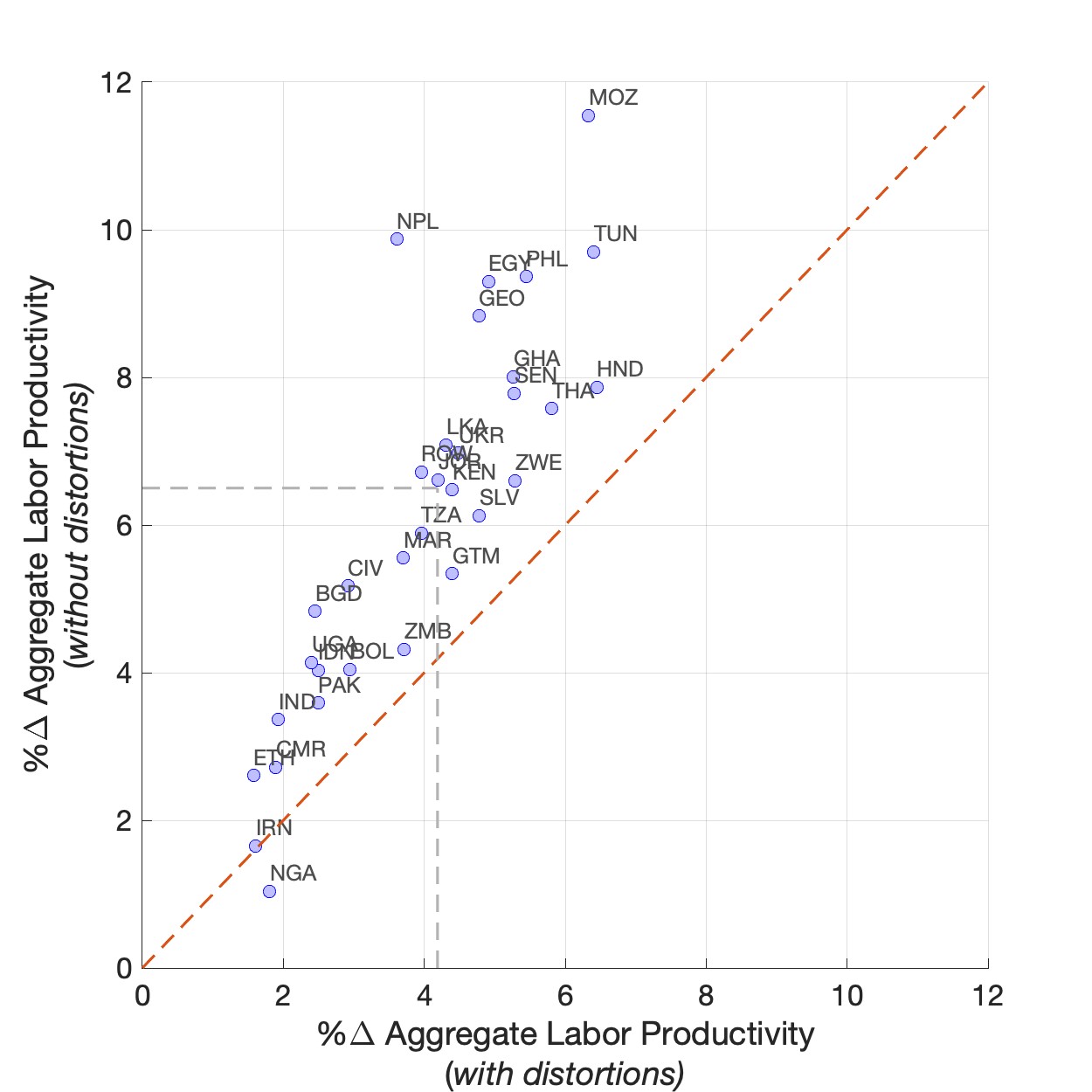 Notes: This figure shows the percentage change to aggregate labor productivity, defined by Equation (), among
low-income countries in response to a 20% reduction in trade costs. The x-axis reports changes under the status quo
labor wedges, the y-axis reports changes under no labor wedges.
Notes: This figure shows the percentage change to aggregate labor productivity, defined by Equation (), among
low-income countries in response to a 20% reduction in trade costs. The x-axis reports changes under the status quo
labor wedges, the y-axis reports changes under no labor wedges.7 Robustness Checks
This section provides robustness checks based on alternative calibrations of our model. First, we use information on formal versus informal firms to assign them to modern and traditional types. Second, we relax the assumption that factor intensities of modern and traditional technologies are common across countries. Third, we experiment with alternative values of the technology elasticity, \(\theta\). Under these alternative calibrations, we re-evaluate the labor productivity effects the trade liberalization discussed in Section 6.2. In addition, this section documents additional empirical patterns and estimates of labor intensity and wedges that support our analysis.
7.1 Formal versus Informal
We adopt here an alternative approach in which we classify firms in the formal sector as modern and firms in the informal sector as traditional. To do so, we bring in the special surveys from the WBES that record firm-level data of the informal sector, the Informal Sector Enterprise Survey (IFS). The surveys on informal firms, however, are available only for 23 countries. Using this subset of countries, we estimate labor intensities and wedges for formal and informal firms. For countries in which this survey is not provided, we use the labor wedges from our baseline calibration. To construct the share of firms and total sales from the informal sector, we use data from Schneider and Buehn (2007), discussed in La Porta and Shleifer (2008). Appendix F.5 provides additional details about the calibration of the model.
There is a large difference between the output elasticity of labor between production technologies in the formal and informal sectors: The output elasticity in the informal sector is 0.53 whereas in the formal sector it is 0.39 (Appendix Figure A.8). In comparison, in our baseline analysis, the output elasticity was 0.39 in the traditional sector against 0.29 in the modern one. Turning to labor market wedges, there is a substantial gap between the average labor wedge in the formal sector (5.04) and that of the informal sector (1.91).In comparison, the average labor wedges in our main calibration were, respectively, 2.28 and 3.69 for traditional and modern firms. That is, the classification based on formal vs. informal divide reinforces the main mechanism in our model as it generates even a larger gap in labor wedges between the resulting two groups of firms. Yet, the correlation between the labor wedges in our baseline analysis and the ones obtained from the formal vs informal cut of the data is 0.83. Importantly, the qualitative patterns that we documented in Section 2 continue to hold under this alternative classification. Simulating the model under this alternative approach, our main quantitative result—that trade liberalization has a larger impact on aggregate labor productivity in efficient economies—is preserved, although the impact becomes somewhat weaker quantitatively (Appendix Figure A.9). 7.2
7.2 Heterogeneous Labor Elasticities across Countries
In our baseline analysis, we assumed that factor intensities of modern and the traditional technologies were common across countries.Two comments are in order regarding this assumption in our baseline analysis. First, production technologies are still different across firms in countries since TFPs vary by firms. Second, the analysis still allows for cross-country differences in aggregate factor intensity as such differences arise from endogenous share of firms that use modern and traditional technologies. Here, we relax this assumption. Because our dataset does not provide us with a sufficient coverage of firms to estimate technology-specific factor intensities separately for each country, as a middle ground, we run our estimation for firms in low-income countries and separately for middle- and high-income countries. This procedure delivers a (potentially) different classification of firms into modern and traditional types, and alternative estimates of output elasticity of labor and labor market wedges.
The output elasticity of labor for each technology is quite comparable between low-income countries and middle- and high-income countries: for low-income countries, the output elasticity of labor in the traditional technology is 0.38, whereas the corresponding elasticity for middle- and high-income countries is 0.41 (Appendix Figure A.8). We find that in both groups of countries labor wedges are larger among modern firms, relative to traditional ones, and this difference is substantially larger among firms in low-income countries—consistent with the pattern in Figure 1 presented earlier in Section 2. Simulating the model with this calibration, we find results that are largely comparable to the ones from our baseline analysis (Appendix Figure A.9). 7.3
7.3 Alternative Values of the Technology Elasticity (\(\theta\))
We conduct two sets of exercises to demonstrate how predictions of our model depend on the technology elasticity, \(\theta\). First, Appendix Figure A.10 shows the results from a 20% reduction in trade costs for different values of \(\theta\). At a higher \(\theta\), the model generates a considerably larger trade-induced adoption of modern technologies. This is expected since a higher technology elasticity implies a larger response when the returns to modern technologies rise (as induced by an improvement in access to foreign intermediates).
However, the effect of the technology elasticity on aggregate labor productivity is less pronounced. On the one hand, an expansion in the use of modern technologies increases aggregate labor productivity. On the other hand (and acting against this force), there is a dampening effect on aggregate productivity because the infra-marginal managerial capital that gets reallocated to the modern technology is less productive than the existing managerial capital there. Numerically, as we increase the technology elasticity, \(\theta\), the relative strength of the former force rises to a limited extent, increasing the impact on the aggregate labor productivity to a modest degree.
Second, we redo our exercise in Section 6.2 with two alternative values of the technology elasticity, \(\theta =2\) and \(\theta =9\) (our baseline calibration sets \(\theta =4.5\)). For these two alternative calibrations, Panels (e)–(h) in Appendix Figure A.9 show the impact of the trade liberalization on aggregate labor productivity and real wages with and without distortions, similar to our main exercise in Section 6.2. The resulting outcomes remain to be similar both qualitatively and quantitatively to our baseline results.
7.4 Additional Evidence
To conclude, we present additional evidence based on the WBES that bolster our quantitative approach.
First, we experiment with several alternative approaches for the estimation of labor intensity and wedges. Specifically, we: (i) estimate labor intensity both by sector and technology type, as opposed to only by technology, (ii) allow for more than 2 technology types, and (iii) estimate labor intensity using different dependent variables (either total sales or total costs) and different control functions. Results are reported in Appendix Table A.1 and Appendix Figures A.1 and A.2. Reassuringly, across all different cuts and estimation approaches, modern firms use labor less intensively than smaller ones, and are subject to higher labor wedges.
Furthermore, we document three patterns using WBES surveys in which firms are asked to report the obstacles they face in their businesses. First, modern firms tend to report more severe obstacles due to taxes, labor regulations and informal sectors relative to traditional firms, but less so in high-income countries (Appendix Table A.2). Second, across several different approaches for the estimation of labor intensity and labor market distortions, modern firms face larger (model-implied) distortions, and more so in low-income countries (Appendix Table A.3). Third, generally our estimates of distortions are positively correlated with these direct measures of obstacles across countries (Appendix Table A.4).
8 Conclusion
In this paper, we studied how labor market imperfections distort firm-level technology choices and alter the gains from trade. To do so, we introduced labor market distortions and technology choices into a multi-country, quantitative trade model. We provided analytical expressions highlighting the mechanisms that drive the impact of trade liberalizations on aggregate welfare and labor productivity. We compared the gains from trade in our framework to the canonical ACR results, and employed counterfactual simulations to study the implications of trade liberalization for aggregate labor productivity, particularly in low-income countries.
Our findings indicates that the low adoption of modern technologies despite globalization, a topic of much debate among researchers and policymakers, can be partly attributed to labor market distortions. Specifically, labor market distortions can substantially reduce the potential labor productivity gains. This is an important result as researchers have been particularly concerned about the implications of technology upgrading for workers, given the stagnation of aggregate labor productivity in parts of the developing world. Our results suggest that reductions in labor market distortions, a ubiquitous feature of developing economies, can substantially boost the labor productivity gains from trade-led growth in modern technologies.
Our paper offers a few promising avenues for future research. First, our framework could be extended to examine the distributional impacts of trade in distorted economies, for example, by bringing in employee-employer matched data on different types of workers. Second, our analysis can be extended to incorporate other forms of inefficiencies, such as barriers that distort firms’ choices of capital. Lastly, our current approach is agnostic about the specific institutional mechanisms that generate labor market distortions. Future research could consider endogenous distortions that interact with technology adoption, for example, by studying the impact of search frictions in labor markets or the implications of moving firms out of informality.
References
References
Acemoglu, D., Antràs, P., and Helpman, E. (2007). Contracts and technology adoption. American Economic Review, 97(3):916–943.
Acemoglu, D. and Zilibotti, F. (2001). Productivity differences. The Quarterly Journal of Economics, 116(2):563–606.
Arkolakis, C., Costinot, A., and Rodriguez-Clare, A. (2012). New trade models, same old gains. American Economic Review, 102(1):94–130.
Artuç, E., Chaudhuri, S., and McLaren, J. (2010). Trade shocks and labor adjustment: A structural empirical approach. American economic review, 100(3):1008–45.
Asturias, J. and Rossbach, J. (2019). Grouped variation in factor shares: An application to misallocation. Available at SSRN 3546842.
Atkin, D. and Donaldson, D. (2021). The role of trade in economic development. Technical report, National Bureau of Economic Research.
Atkin, D. and Khandelwal, A. K. (2020). How distortions alter the impacts of international trade in developing countries. Annual Review of Economics, 12:213–238.
Bai, Y., Jin, K., and Lu, D. (2019). Misallocation under trade liberalization. Technical report, National Bureau of Economic Research.
Baqaee, D. and Farhi, E. (2019). Networks, barriers, and trade. Technical report, National Bureau of Economic Research.
Bartelme, D. G., Costinot, A., Donaldson, D., and Rodriguez-Clare, A. (2019). The textbook case for industrial policy: Theory meets data. Technical report, National Bureau of Economic Research.
Basu, S. and Weil, D. N. (1998). Appropriate technology and growth. The Quarterly Journal of Economics, 113(4):1025–1054.
Bernard, A. B. and Jensen, J. B. (1999). Exceptional exporter performance: cause, effect, or both? Journal of international economics, 47(1):1–25.
Bernard, A. B., Jensen, J. B., Redding, S. J., and Schott, P. K. (2007). Firms in international trade. Journal of Economic perspectives, 21(3):105–130.
Bertrand, M., Hsieh, C.-T., and Tsivanidis, N. (2021). Contract labor and firm growth in india. Technical report, National Bureau of Economic Research.
Besley, T. and Burgess, R. (2004). Can labor regulation hinder economic performance? evidence from india. The Quarterly journal of economics, 119(1):91–134.
Buera, F. J., Hopenhayn, H., Shin, Y., and Trachter, N. (2021). Big push in distorted economies. Technical report, National Bureau of Economic Research.
Bustos, P. (2011). Trade liberalization, exports, and technology upgrading: Evidence on the impact of mercosur on argentinian firms. American economic review, 101(1):304–40.
Caliendo, L., Dvorkin, M., and Parro, F. (2019). Trade and labor market dynamics: General equilibrium analysis of the china trade shock. Econometrica, 87(3):741–835.
Caliendo, L., Parro, F., and Tsyvinski, A. (2017). Distortions and the structure of the world economy. Technical report, National Bureau of Economic Research.
Ciccone, A. (2002). Input chains and industrialization. The Review of Economic Studies, 69(3):565–587.
Costinot, A. and Rodríguez-Clare, A. (2014). Trade theory with numbers: Quantifying the consequences of globalization. In Handbook of international economics, volume 4, pages 197–261. Elsevier.
Davidson, C., Matusz, S. J., and Shevchenko, A. (2008). Globalization and firm level adjustment with imperfect labor markets. Journal of international Economics, 75(2):295–309.
De Loecker, J., Goldberg, P. K., Khandelwal, A. K., and Pavcnik, N. (2016). Prices, markups, and trade reform. Econometrica, 84(2):445–510.
Dekle, R., Eaton, J., and Kortum, S. (2007). Unbalanced trade. American Economic Review, 97(2):351–355.
Diao, X., Ellis, M., McMillan, M. S., and Rodrik, D. (2021). Africa’s manufacturing puzzle: Evidence from tanzanian and ethiopian firms. Technical report, National Bureau of Economic Research.
Ding, S., Lashkaripour, A., and Lugovskyy, V. (2023). A global perspective on the incidence of monopoly distortions.
Dix-Carneiro, R., Goldberg, P. K., Meghir, C., and Ulyssea, G. (2021). Trade and informality in the presence of labor market frictions and regulations. Technical report, National Bureau of Economic Research.
Eaton, J. and Kortum, S. (2002). Technology, geography, and trade. Econometrica, 70(5):1741–1779.
Farrokhi, F. and Pellegrina, H. S. (2023). Trade, technology, and agricultural productivity. Journal of Political Economy, 131(9).
Farrokhi, F. and Soderbery, A. (2023). Trade elasticities in general equilibrium: Demand, supply, and aggregation.
Fieler, A. C. (2011). Nonhomotheticity and bilateral trade: Evidence and a quantitative explanation. Econometrica, 79(4):1069–1101.
Fieler, A. C., Eslava, M., and Xu, D. Y. (2018). Trade, quality upgrading, and input linkages: Theory and evidence from colombia. American Economic Review, 108(1):109–46.
Foster, L., Haltiwanger, J., and Krizan, C. J. (2006). Market selection, reallocation, and restructuring in the us retail trade sector in the 1990s. The Review of Economics and Statistics, 88(4):748–758.
Goldberg, P. K., Khandelwal, A. K., Pavcnik, N., and Topalova, P. (2010). Imported intermediate inputs and domestic product growth: Evidence from india. The Quarterly journal of economics, 125(4):1727–1767.
Haltiwanger, J., Scarpetta, S., and Schweiger, H. (2014). Cross country differences in job reallocation: The role of industry, firm size and regulations. Labour Economics, 26:11–25.
Hashemi, A., Kirov, I., and Traina, J. (2022). The production approach to markup estimation often measures input distortions. Economics Letters, 217:110673.
Hopenhayn, H. and Rogerson, R. (1993). Job turnover and policy evaluation: A general equilibrium analysis. Journal of political Economy, 101(5):915–938.
Hsieh, C.-T. and Klenow, P. J. (2009). Misallocation and manufacturing tfp in china and india. The Quarterly journal of economics, 124(4):1403–1448.
Hsieh, C.-T. and Klenow, P. J. (2014). The life cycle of plants in india and mexico. The Quarterly Journal of Economics, 129(3):1035–1084.
Imbs, J. and Mejean, I. (2015). Elasticity optimism. American Economic Journal: Macroeconomics, 7(3):43–83.
Kucheryavyy, K., Lyn, G., and Rodríguez-Clare, A. (2023). Grounded by gravity: A well-behaved trade model with industry-level economies of scale. American Economic Journal: Macroeconomics, 15(2):372–412.
La Porta, R. and Shleifer, A. (2008). The unofficial economy and economic development. Technical report, National Bureau of Economic Research.
La Porta, R. and Shleifer, A. (2014). Informality and development. Journal of economic perspectives, 28(3):109–126.
Lagakos, D. (2016). Explaining cross-country productivity differences in retail trade. Journal of Political Economy, 124(2):579–620.
Lanteri, A., Medina, P., and Tan, E. (2023). Capital-reallocation frictions and trade shocks. American Economic Journal: Macroeconomics, 15(2):190–228.
Lashkaripour, A. and Lugovskyy, V. (2023). Profits, scale economies, and the gains from trade and industrial policy. American Economic Review, 113(10):2759–2808.
Levinsohn, J. and Petrin, A. (2003). Estimating production functions using inputs to control for unobservables. The review of economic studies, 70(2):317–341.
Lucas, R. E. (1978). On the size distribution of business firms. The Bell Journal of Economics, pages 508–523.
Medina, P. (2020). Import competition, quality upgrading and exporting: Evidence from the peruvian apparel industry. University of Toronto mimeo.
Meghir, C., Narita, R., and Robin, J.-M. (2015). Wages and informality in developing countries. American Economic Review, 105(4):1509–1546.
Midrigan, V. and Xu, D. Y. (2014). Finance and misallocation: Evidence from plant-level data. American economic review, 104(2):422–58.
Morlacco, M. (2019). Market power in input markets: Theory and evidence from french manufacturing. Unpublished, March, 20:2019.
Murphy, K. M., Shleifer, A., and Vishny, R. W. (1989). Industrialization and the big push. Journal of political economy, 97(5):1003–1026.
Oberfield, E. (2013). Productivity and misallocation during a crisis: Evidence from the chilean crisis of 1982. Review of Economic Dynamics, 16(1):100–119. Special issue: Misallocation and Productivity.
Olley, G. S. and Pakes, A. (1996). The dynamics of productivity in the telecommunications equipment industry. Econometrica, 64(6):1263–1297.
Pavcnik, N. (2017). The impact of trade on inequality in developing countries. Technical report, National Bureau of Economic Research.
Ramondo, N. and Rodríguez-Clare, A. (2013). Trade, multinational production, and the gains from openness. Journal of Political Economy, 121(2):273–322.
Schneider, F. and Buehn, A. (2007). Shadow economies and corruption all over the world: revised estimates for 120 countries. economics, 1(1).
Scottini, L. C. (2018). Firm-level distortions, trade, and international productivity differences. Unpublished manuscript.
Simonovska, I. and Waugh, M. E. (2014). The elasticity of trade: Estimates and evidence. Journal of international Economics, 92(1):34–50.
Sotelo, S. (2020). Domestic trade frictions and agriculture. Forthcoming in Journal of Political Economy.
Ulyssea, G. (2018). Firms, informality, and development: Theory and evidence from brazil. American Economic Review, 108(8):2015–47.
Verhoogen, E. (2021). Firm-level upgrading in developing countries.
Yeaple, S. R. (2005). A simple model of firm heterogeneity, international trade, and wages. Journal of international Economics, 65(1):1–20.
Zavala, L. (2022). Unfair trade? monopsony power in agricultural value chains.
Part
Appendices
Online Appendices for “Trade and Technology Adoption in Distorted Economies”
Not for Publication
Farid Farrokhi, Ahmad Lashkaripour, and Heitor S. PellegrinaEmail: ffarrokh@purdue.edu, alashkar@indiana.edu, and hpelleg@nd.edu.
A Derivations of Model Relationships and ALP
This section presents, first, derivations that relate model-implied revenue shares, labor shares, and the share of modern firms. We use these relationships throughout the paper to derive several of our expressions. In addition, we present a full derivation of our formula for aggregate labor productivity.
A.1 Relationship between \(\alpha\), \(\rho\), and \(\ell\)
This appendix derives expressions for revenue shares (\(\rho _{i,st}\)) and labor shares (\(\ell _{i,st}\)) as a function of \(\alpha _{i,st}\), which is the share of firms that chose technology \(t\) in country \(i\)–industry \(s\). To fix idea, we formally define the aforementioned share variables. The labor shares are defined as follows for various tiers of production (i.e., firm, technology, and industry)
We use \(\rho\) to denote within-industry revenue shares and \(r\) to denote industry-level revenue share. In particular,
where \(R_{i,st}\left (\omega \right )\equiv p_{i,s}Q_{i,st}\left (\omega \right )\), recall, denotes total revenues collected by firm \(\omega\), with \(R_{i,s}\equiv \sum _{t}\int _{\omega }R_{i,st}\left (\omega \right )dF\left (\omega |\omega \in \Omega _{st}\right )\) denoting industry-level revenues. Appealing to Equations () and (2) we can derive the following relationship between firm and sales shares:
Combining the above equation with the adding up constraints, \(\sum _{t}\rho _{i,st}=\sum _{t}\alpha _{i,st}=1\), yields
To derive a relationship between labor shares and firm shares, we appeal to the fact that gross labor cost equals a constant fraction, \(\gamma _{st}^{L}\), of gross revenues. In particular,
Combining this equation with the adding up constraints, \(\sum _{t}\ell _{i,st}=\ell _{i,s}\) and \(\sum _{t}\alpha _{i,st}=1\), delivers
A.2 Aggregate Labor Productivity (ALP)
We define Aggregate Labor Productivity (ALP) at the level of country-industry-technology as output per worker there. Using the relationship between revenues and quantities as well as the labor market clearing condition, it follows that:
Similarly, ALP at the level of industry can be expressed as:
Lastly, we derive the expression for ALP at the level of country. Here, we aggregate over industry-level output quantities using the final consumption aggregator, \(Q_{i}=\prod _{s}\left (Q_{i,s}\right )^{\beta _{i,s}}\). Under this assumption, we have:
where \(\ell _{i,st}\equiv \frac {L_{i,st}}{L_{i}}\) and \(\pi _{ii,s}\) is the domestic expenditure share. In the above, we use \(P_{i,s}=p_{i,s}\left (\pi _{ii,s}\right )^{\frac {1}{\sigma _{s}-1}}\) and \(P_{i}=\prod _{s}P_{i,s}^{\beta _{i,s}}.\)
To establish the relationship between aggregate labor productivity \(\text{ALP}_{i}\) (Equation ) and welfare \(W_{i}\) (Equation 9), start from the third line of the above derivation, and replace for \(\text{ALP}_{i,st}=\frac {R_{i,st}}{p_{i,s}L_{i,st}},\)
Denoting \(Y_{i,s}\) as total value added and \(\bar {\gamma }_{i,s}^{M}\) as the average cost share of intermediate inputs in country \(i-\) industry \(s\), using the relationship between producer and consumer prices (as shown above), and definition of welfare \(W_{i}=Y_{i}/P_{i}\), we can express \(\text{ALP}_{i}\) as:
B General Equilibrium in Changes
B.1 Specifying the System of GE in Changes
Consider a “policy” as a set of exogenous shocks to trade costs, labor wedges, and productivities, \(\mathscr {P}=\{\hat {d}_{ij,s},\hat {\tau }_{i,st}^{L},\hat {a}_{i,st}\}\). Let \(\mathscr {B}=\{\sigma,\theta,\pi _{ij,s},\alpha _{i,st},\gamma _{st}^{L},\gamma _{st}^{M},\gamma _{st}^{Z},\tau _{i,st}^{L},\phi _{i,\ell s},\beta _{i,s},w_{i}L_{i},R_{i,st},E_{i,s},Y_{i}\}\) denote the “baseline” values of the general equilibrium—i.e., the set of sufficient statistics. For any generic variable \(x\) in the baseline equilibrium, let \(x^{\prime }\) be its corresponding value in the counterfactual equilibrium, and \(\hat {x}\equiv x^{\prime }/x\) denote its change from the baseline to the counterfactual equilibrium. Given policy \(\mathscr {P}\) and baseline values \(\mathscr {B}\), the following equations define general equilibrium in changes to trade and technology shares, aggregate sales and expenditures, and prices and wages, \(\mathscr {E}\equiv \{\hat {\pi }_{ij,s},\hat {\alpha }_{i,st},\hat {R}_{i,st},\hat {E}_{i,s},\hat {Y}_{i},\hat {p}_{i,s},\hat {P}_{i,s},\hat {w}_{i}\}\).
The change to sales in country \(i-\) industry \(s-\) technology \(t\) is:
where the change to the share of firms in each technology type is given by:
and the change to technology-specific return to managerial capital is:
In turn, the change to the industry-level (consumer) price index equals:
and the change to within-industry share of expenditure (trade share) is:
Lastly, the following four equations guarantee the market clearing conditions and the accounting of general equilibrium. The labor market clearing condition and the goods market clearing condition in the counterfactual equilibrium must satisfy:
The change to the industry-level gross expenditures and the total national expenditure (nominal GDP) satisfy:
We now turn to presenting the computational algorithm that we use to simulate the general equilibrium of our model in response to counterfactual policy shocks.
B.2 Numerical Algorithm to Simulate the GE in Changes.
- Guess \(\widehat {w}_{i}\) and \(\widehat {p}_{i,s}\). (By the choice of numeraire, here we impose that \(\hat {w}_{i_{0}}=1\) for a reference country \(i_{0}\))
- Calculate the change to industry-level price index, \(\widehat {P}_{i,s}\), according to Equation (B.4).
- Calculate the change to technology-level returns to managerial capital according to Equation (B.3).
- Calculate the change to trade shares, \(\hat {\pi }_{ij,s}\), based on Equation (B.5).
- Calculate the change to technology shares, \(\widehat {\alpha }_{i,st}\), according to Equation (B.2).
- Calculate the change to sales, \(\hat {R}_{i,st}\), based on Equation (B.1).
- Calculate the change to national expenditure, \(\hat {Y}_{i}\), based on Equation (B.9).
- Calculate the change to industry-level gross expenditures, \(\widehat {E}_{i,s}\), based on Equation (B.8).
Update the change to wages and prices, based on market clearing conditions (B.6) and (B.7),
\[\left (\widehat {w}_{i}\right )^{new}=\frac {1}{w_{i}L_{i}}\left [\sum _{s,t}\frac {\gamma _{st}^{L}}{\hat {\tau }_{i,st}^{L}\tau _{i,st}^{L}}\widehat {R}_{i,st}R_{i,st}\right ]\]\[\left (\widehat {p}_{i,s}\right )^{new}=\frac {\sum _{j}\hat {\pi }_{ij,s}\pi _{ij,s}\hat {E}_{j,s}E_{j,s}}{\left (\sum _{t}\left (\hat {R}_{i,st}/\hat {p}_{i,st}\right )R_{i,st}\right )}\]If the \(|\left (\widehat {w}_{i}\right )^{new}-\widehat {w}_{i}|>\epsilon\) and \(|\left (\widehat {p}_{i,s}\right )^{new}-\widehat {p}_{i,s}|>\epsilon\), for a sufficiently small tolerance \(\epsilon\), then update: \(\widehat {w}_{i}=\left (\widehat {w}_{i}\right )^{new}\) and \(\hat {p}_{i,s}=\left (\widehat {p}_{i,s}\right )^{new}\), and normalize the updated price and wage changes with respect to the wage change in a reference country (whose labor serves as a numeraire), then go to Step 2. Otherwise, the convergence is achieved.
C Derivation of The Welfare Cost of Misallocation
Consider the closed economy case of our model with one sector and multiple technologies—noting that, with a reinterpretation of indexes, our derivation extends to multiple sectors and technologies. We, accordingly, condense the notation by dropping the industry subscript, \(s\), going forward. To provide closed-form formulas for the degree of misallocation, we make two additional assumptions: First, we assume that production employs only primary factors of production—namely, labor and managerial capital. Second, we assume that the labor intensity parameter, \(\gamma _{i,t}^{L}\), is common across technologies. All in all, we consider a closed economy where production can be conducted under multiple technologies with different labor input wedges, with firms having the ability to choose and adjust their preferred technology.
Intermediate Definitions.The efficient allocation in this stylized version of our model is achieved if labor input wedges and the revenue associated with them are eliminated from the economy—which is akin to analyzing the following shock:
Let \(\hat {W}_{i}\left (\hat {\boldsymbol {\tau }}_{i}\right )\) denote the resulting welfare change from the wedge reduction shock, \(\hat {\boldsymbol {\tau }}_{i}\equiv \left \{ \tau _{i,t}^{L}\right \}\). We define the degree of misallocation (\(\mathcal {D}_{i}\)) as the welfare distance between the decentralized (i.e, misallocated) and the efficient economies. Namely,
The Change in Technology Composition.Considering our assumption that \(\gamma _{i,t}^{L}=\gamma _{i,t'}^{L}=\gamma _{i}^{L}\) and \(\gamma _{i,t}^{Z}=\gamma _{i,t'}^{Z}=\gamma _{i}^{Z}\) for all \(t\) and \(t'\), we can specify the change in the share of firms choosing technology \(t\) as
Appealing to the above expression, we can characterize the change in technology-level employment shares. For this, we invoke the relationships derived in Appendix A.1 to arrive at
Notice that in the efficient, wedge-free equilibrium, employment and revenue shares exactly coincide with firm shares (i.e., \(\ell '_{i,t}=\rho '_{i,t}=\alpha '_{i,t}\)), yielding the following expression for technology-level employment shares in the counterfactual wedge-free equilibrium:
The Change in Nominal Income.In the decentralized (baseline) economy, nominal income in country \(i\) is the sum of wage income, managerial rents, and wedge revenues—i.e., \(Y_{i}=w_{i}L_{i}+\Pi _{i}+T_{i}\). Noting that \(w_{i}L_{i}+T_{i}=\sum _{t}\tau _{i,t}^{L}w_{i}L_{i,t}\) and that by cost minimization, \(\Pi _{i}=\sum _{t}\frac {\gamma _{i}^{Z}}{\gamma _{i}^{L}}\tau _{i,t}^{L}w_{i}L_{i,t}\), we can specify the nominal income in the baseline economy as
Invoking the same logic, nominal income in the efficient (counterfactual) economy is \({Y'}_{i}=\sum _{t}\left [\frac {1}{\gamma _{i}^{L}}\ell '_{i,t}\right ]{w'}_{i}L_{i}\). Combining the expressions for \(Y_{i}\) and \({Y'}_{i}\) and assigning labor in country \(i\) as the numeraire (\({w'}_{i}=w_{i}=1\)) deliver the following expression for the change in nominal income in country \(i\):
Finally, appealing to our short-hand notation for weighted means, \(\mathbb {E}_{\ell }\left [\tau _{i,t}^{L}\right ]=\sum _{t}\left [\tau _{i,t}^{L}\ell _{i,t}\right ]\), we can express the change in log income as:
The Change in Consumer Prices.Following Equation (2) in Section 3, the change in the competitive price of goods produced via technology \(t\) is
where the above equation uses two features of our stylized model: First, \(\hat {\Gamma }_{i}^{Z}=1\), since factor intensities are the same across technologies. Second, gross output, \(R_{i}\), equals value added, \(Y_{i}\), since no intermediate inputs are used in production—and, hence, in a one-sector economy \(R_{i}=Y_{i}\) delivers national income. By choice of numeraire, \(\hat {w}_{i}=1\), and using Equation (1), we can express the change in \(H_{i}\) as:
Plugging the above expression back into Equation (C.3) yields
Using ourshort-hand notation for means, whereby \(\mathbb {E}_{\alpha }\left [\left (\tau _{i,t}^{L}\right )^{\frac {\gamma _{i}^{L}}{\gamma _{i}^{Z}}\theta }\right ]=\sum _{t'}\left [\alpha _{i,t'}\left (\tau _{i,t'}^{L}\right )^{\frac {\gamma _{i}^{L}\theta }{\gamma _{i}^{Z}}}\right ]\) and noting that \(\hat {Y_{i}}=\mathbb {E}_{\ell }\left [\tau _{i,t}^{L}\right ]^{-1}\) (Equation (C.2)), we get
where thefirst mean on the right-hand side can be converted from an \(\alpha\)-weighted mean to an \(\ell\)-weighted mean by noticing that \(\alpha _{i,t}=\tau _{i,t}\ell _{i,t}/\mathbb {E}_{\ell }\left [\tau _{i,t}\right ]\) . Specifically,
which when plugged into our last expression for \(\hat {p}_{i}\), yields
Assembling the Pieces Together.The final step collects the expressions for \(\hat {Y}_{i}\) (Equation (C.2)) and \(\hat {p}_{i}\) (Equation ()), to calculate the degree of misallocation, \(\mathcal {D}_{i}=\log \hat {Y}_{i}-\log \hat {P}_{i}\) . Doing so and rearranging the terms delivers,
where, recall that, \(\tilde {\tau }_{i,t}\equiv \tau _{i,t}/\mathbb {E}_{\ell }[\tau _{i,t}]\).
Next, we reintroduce the sector subscript, \(s\), for consistency in notation, implicitly assuming that all sectors are symmetric. We also substitute \(\gamma _{i}^{L}\) and \(\gamma _{i}^{Z}\) with our notation for average input intensities, \(\bar {\gamma }_{i}^{L}\), and \(\bar {\gamma }_{i}^{Z}\)—noting that the average input intensities are the same as \(\gamma _{i}^{L}\) and \(\gamma _{i}^{Z}\) when sectors are symmetric. With these amendments to the notation, we get the following expression for the welfare cost of misallocation:
Later, we invoke this formula to characterize the cost of misallocation in the presence of multiple asymmetric sectors that differ in their factor intensities. Before that, we provide a first-order approximation for \(\mathcal {D}_{i}\) to elucidate the determinants of misallocation.
Approximate Formula.Next, we derive a simple approximation for \(\mathcal {D}_{i}\) using Taylor’s Theorem. To this end, we construct the Taylor expansion of the following function,
around \(\left \{ \tilde {\tau }_{i,st}^{L}\right \} =\left \{ 1,...,1\right \}\), which delivers the following second-order approximation
Notice that \(\mathbb {E}_{\ell }\left [\tilde {\tau }_{i,st}^{L}\right ]=1\) since \(\tilde {\tau }_{i,st}\equiv \tau _{i,st}/\mathbb {E}_{\ell }\left [\tau _{i,st}^{L}\right ]\). Also, the second term on the right-hand is zero by definition of the mean and the last term is simply the variance of \(\left \{ \tilde {\tau }_{i,st}^{L}\right \} _{t}\), which we denote by \(\text{Var}_{\ell }\left [\tilde {\tau }_{i,st}^{L}\right ]\). Considering these points we can simplify the above approximation as
Plugging the above approximation back into Equation C.4 and noting that \(\log \left (1+x\right )\approx x\) when \(x\approx 0\), we get
C.1 Cost of Misallocation with Multiple Sectors
Next, we consider an economy with multiple sectors that differ in their labor intensities. The change in nominal income is still given by \(\hat {Y}_{i}=\mathbb {E}_{\ell }\left [\tau _{i,st}^{L}\right ]^{-1}\). Following our earlier derivations, the change in sector-level prices are given by
which, considering that \(\hat {Y}_{i}=\mathbb {E}_{\ell }\left [\tau _{i,st}^{L}\right ]^{-1}\) and our notation for the mean operator, yields
Notice that with multiple sectors \(\alpha _{i,st}=\tau _{i,st}\ell _{i,st}/\mathbb {E}_{\ell,s}\left [\tau _{i,st}^{L}\right ]\), where \(\mathbb {E}_{\ell,s}\left [.\right ]\) denotes the within-industry mean weighted by industry \(s\) employment shares. Appealing to the point, we can re-write the first mean on the right-hand side of the above equation as
Combining the above two equations, derivers the following expression for the change in real income with respect to industry \(s\) goods:
To make the notation more compact, redefine the normalized wedges at the technology and industry levels as
Finally, given that preferences are Cobb-Douglas across industries \(\mathcal {D}_{i}=\sum _{s}e_{i,s}\log \left (\frac {\hat {Y}_{i}}{\hat {p}_{i,s}}\right )\), which delivers the following equation for the welfare cost of misallocation in a multi-sector model:
D Derivations of Trade Effects on Welfare and Labor Productivity
In this section, we derive the equations presented in Section 4.2.1 of the paper, which specify the impacts of trade on welfare and the labor productivity gains. We first employ the exact hat algebra to derive exact welfare formulas. Moreover, to draw additional insight into the mechanisms behind welfare effects, we also produce local approximations from our exact formulas.
D.1 Exact Changes to Income Levels and Prices
For any generic variable \(x\) in the baseline equilibrium let \(x'\) be the corresponding value in the counterfactual equilibrium, with the hat variable denoted by \(\hat {x}\equiv x'/x\). Consider a set of shocks to trade costs, \(\left \{ \hat {d}_{ij,k}\right \}\), and labor wedges, \(\left \{ \hat {\tau }_{i,st}^{L}\right \}\). The welfare impact of these shocks can be written as the change in national income divided by the change in the final consumer price index,
Similarly, the change to the real wage is given by:
We now turn to characterizing the change to income levels, wage bills, and prices.
Change in Income.Recall that national income is the sum of net wage payments, the revenue associate with labor wedges, and rents accruing to managerial capital. Namely, \(E_{i}=w_{i}L_{i}+T_{i}+\Pi _{i}\), where \(T_{i}\equiv \sum \left [\left (\tau _{i,st}^{L}-1\right )w_{i}L_{i,s}\right ]\) is the revenue from wedges and \(\Pi _{i}\equiv \sum _{s,t,\omega }\Pi _{i,st}\left (\omega \right )\) is the sum of managerial rents. Since \(w_{i}L_{i}+T_{i}=\sum _{s}\sum _{t}\left [\tau _{i,st}^{L}\ell _{i,st}\right ]w_{i}L_{i}\) and \(\Pi _{i}=\frac {\gamma _{st}^{Z}}{\gamma _{st}^{L}}\left (w_{i}L_{i}+T_{i}\right )\), we can express country \(i\)’s level of income as:
where \(\ell _{i,st}\equiv L_{i,st}/L_{i}\). Therefore, the change to income can be expressed as:
where \(y_{i,st}\) is the share of income in country \(i\) that is generated in industry \(s-\) technology \(t\),
Change in Prices.Using Equation () from the main text, the change to output (sales) from country \(i-\) industry \(s-\) technology \(t\) , \(\hat {R}_{i,st}\), equals:
Moreover, it follows from Equation (1) that the change to returns per dollar of output in country \(i-\) industry \(s-\) technology \(t\), \(\hat {h}_{is,t}\), is given by:
Replacing \(\widehat {h}_{i,st}\) from Equation (D.4) into Equation (D.3) delivers the following expression for \(\hat {R}_{i,s,t}\):
The above formula represents the supply in terms of sales as a function of price (moving along the curve) and other variables (shifting the curve). The inverse supply function will then represents the change to producer price as a function of output, and all the shifters,
Since \(\gamma _{st}^{L}R_{i,st}=\tau _{i,st}w_{i}\ell _{is,t}L_{i}\), we can express the change to output, \(\hat {R}_{i,st}\), as:
Moreover, the change to price index of the intermediate input bundle can be written as:
where \(\phi _{i,ss'}\) denotes the share corresponding to origin industry \(s'\) and destination industry \(s\), with \(\sum _{s'}\phi _{i,ss'}=1\). Replacing from Equations (D.6) and (D.7) into Equation (D.5), the change to produce price can be expressed in the following way:
It follows from the CES demand structure that the industry-level consumer price index equals \(\hat {P}_{i,s}=\hat {p}_{i,s}\times \left (\hat {\pi }_{ii,s}\right )^{\frac {1}{\sigma _{s}-1}}\) , which implies \(\hat {p}_{i,s}=\hat {P}_{i,s}\times \left (\hat {\pi }_{ii,s}\right )^{-\frac {1}{\sigma _{s}-1}}\). Replacing for \(\hat {p}_{i,s}\), taking logs, using the output shares \(\rho _{i,st}\) (with \(\sum _{t}\rho _{i,st}=1\)), and noting that \(\gamma _{st}^{L}+\gamma _{st}^{Z}=1-\gamma _{st}^{M}\), the change to the industry-level consumer price index, \(\hat {P}_{i,s}\), can be expressed as:
where \(B_{i,s}\) is given by:
and, \(\bar {\gamma }_{i,s}^{M}\equiv \sum _{t}\rho _{i,st}\gamma _{st}^{M}=\sum _{t}\frac {R_{i,st}}{R_{i,s}}\gamma _{st}^{M}\) is the aggregate share of intermediates in gross output of country \(i-\) industry \(s\). Equation (D.8) forms a linear system of equations which can be expressed more compactly in the matrix format as:
The solution to this system of equations is given by:
The above solution delivers the industry-level consumer price index as \(\ln \hat {P}_{i,s}=\sum _{k}\varphi _{i,sk}B_{i,k}\),which can be expanded as:
Note, to arrive at the above formula we have used the fact that \(\sum _{k}\varphi _{i,sk}\left (1-\bar {\gamma }_{i,k}^{M}\right )=1\).
Using Equation (), we can now express the log final consumer price index in the following way:
Converting the log variables to level variables, the exact change to the final consumer price index equals:
Integrating Change in Income and Prices.By combining the change in income from Equation (D.1) and change in the consumer price index from Equation (D.9), the change to welfare can be expressed as:
D.2 Ex-Ante Welfare Gains from Trade Liberalization
Consider a set of local shocks only to trade costs of country \(i\), keeping all other exogenous parameters (including labor wedges) unchanged. First, we derive the local change to income. Note that the log income change can be written as the change associated with wage bills and wedge revenues plus the one from managerial rents:
Replacing for
and, noting that \(\text{d}\ln \Pi _{i,st}=\text{d}\ln w_{i}+\text{d}\ln \ell _{i,st}\), we obtain:
where \(\bar {\gamma }_{i}^{L}\equiv \sum _{s,t}\left [\frac {R_{i,st}}{R_{i}}\gamma _{st}^{L}\right ]\) is the aggregate share of wage bills in gross output of country \(i\). Similarly, and as before, \(\bar {\gamma }_{i}^{M}\equiv \sum _{s,t}\left [\frac {R_{i,st}}{R_{i}}\gamma _{st}^{L}\right ]\) is the aggregate share of intermediates in gross output of country \(i\).
Next, we derive the local change to log consumer price index. Note, for an exact change in any generic variable \(x\), denoted by \(\hat {x}\equiv \frac {x^{\prime}}{x}=1+\frac {\text{d}x}{x}\), the following first order approximation can be used to convert (\(\hat {x}\)) into (\(\text{d}\ln x\)),
We can, therefore, use Equation (D.9) to express the change in log consumer price index:
where \(\varphi _{i,sk}\) corresponds to entry \(\left (s,k\right )\) of country \(i\)’s Leontief inverse matrix.
By combining the change in log income from Equation (D.11) and change in log consumer price index from Equation (D.12), we can derive the change to welfare as:
where \(\Lambda _{i,s}\equiv p_{i,s}Q_{i,s}/Y_{i}\) is the Domar weight for industry \(s\). The above equation reproduce Equation () in the main text.
Additionally, let us produce the above formula in the special case of our model in which the economy consists of a single sector. In that case, \(\beta _{i,s}\equiv \beta _{i}=1\), \(\varphi _{i,sk}\equiv 1/(1-\bar {\gamma }_{i}^{M})\), and \(\Lambda _{i,k}\equiv \Lambda _{i}=1/(1-\bar {\gamma }_{i}^{M})\). Hence,
Note that a portion of the ToT effects associated with changes in rental rate of managerial capital disappear since (\(\Lambda _{i,k}-\sum _{s}\beta _{i,s}\varphi _{i,sk}=0\)) in the one-sector economy.
D.3 Ex-Post Welfare Gains from Trade
In this subsection, we derive the ex post welfare gains from trade, as the loss of real national income of each country \(i\) if it is moved from autarky to the baseline (observed) equilibrium. For communicating forces at play as clearly as possible, we consider the single-sector version of our model.
To begin, consider any trade cost shock. It follows from Equation (2) in the main text that the change to the produce price is:
In turn, using Equation (1), the change in the returns to managerial capital equals:
In the single-industry version of the model, which we consider here, the price index of the intermediate input is the same as the consumer price index, i.e., \(\hat {m}_{i}=\hat {P}_{i}\). In addition, the CES demand structure connects the producer and consumer prices, \(\hat {p}_{i}=\hat {P}_{i}\left (\hat {\pi }_{ii}\right )^{-\frac {1}{\sigma -1}}\). Replacing for these relationships into Equation (D.14), we can rewrite the change to technology-specific managerial returns as:
Next, note that labor market clearing condition in country \(i\) can be expressed as \(w_{i}L_{i}=\Gamma _{i}^{L}\times Y_{i}\), where \(\Gamma _{i}^{L}\equiv \sum _{t}\left (\gamma _{t}^{L}/\tau _{i,t}^{L}\right )\rho _{i,t}\) . Using this equation, we can relate the change in wage to change in income:
where \(\hat {\Gamma }_{i}^{L}\) will be specified below. Integrating Equations (D.15) and (D.16), the following expression reorganizes the change to welfare, \(\hat {W_{i}}=\hat {Y}_{i}/\hat {P}_{i}\),
Equation (D.17) indirectly represents the change to welfare, \(\hat {W_{i}}\), in response to any shock to trade costs of the country which is considered. As it is evident from the formula (unless \(\gamma _{t}^{Z}\) and \(\gamma _{t}^{L}\) are invariant between the two technology types) there is generally no closed-form solution to \(\hat {W}_{i}\).
To make progress, let us focus on the specific case of autarkic counterfactual which corresponds to: \(\hat {\pi }_{ii}=1/\pi _{ii}\), where \(\pi _{ii}\) denotes the baseline domestic expenditure share. We can express the gains from trade, \(\text{GT}_{i}\), as the loss in real income when country \(i\) is moved from its baseline equilibrium to autarky:
where the country-specific multiplier, \(\Delta _{i}\), solves the following equation:
Here, \(\hat {\Gamma }_{i,t}\) summarizes the welfare-relevant change in factor intensities across the technology types. Specifically, note that
Given Equations (D.20) and (D.21), we can calculate \(\hat {\Gamma }_{i,t}\) according to the following equation:
where the change to technology shares are, \(\hat {\alpha }_{i,t}\), is given by:
Taking stock, the country-specific multiplier, \(\Delta _{i}\), along with \(\left (\widehat {\Gamma }_{i}^{Z},\widehat {\Gamma }_{i}^{L},\widehat {\Gamma }_{i,t},\hat {\alpha }_{i,t}\right )\) are the solutions to Equation (D.19), (D.20), (D.21), (D.22) and (D.23).
Gains from Trade in ACR Model.It is instructive to benchmark the gains from trade in our model to the ACR formula. Consider a special case of our model in which production in each industry is restricted to use only one type of technology, \(\alpha _{i,s0}=1\) and \(\alpha _{i,s1}=0\). In that case, there will be no change in the share of firms and employment across technologies \(\hat {\alpha }_{i,st}=\hat {\ell }_{i,st}=1\). Using Equations (D.10) and (), setting \(\hat {\tau }_{i,st}^{L}=1\) (no change in labor distortions) and \(\hat {\pi }_{ii,s}=1/\pi _{ii,s}\) (moving to autarky) the GFT in our model reduces to the ACR formula:
D.4 Ex-Ante Labor Productivity Gains from Trade Liberalization
Using Equation (), we can write down the change to (log) aggregate labor productivity (ALP) of country \(i\) as:
Define
Therefore, we can rewrite the above formula for ALP as:
In addition, using Equation (), the change to (log) real wage can be expressed as:
Combining Equations (D.24) and (D.25),
In a single-sector version of the model, expenditure shares collapse to unity \(\beta _{i,k}\equiv \beta _{i}=1\), and the entries of the Leontief inverse matrix are \(\varphi _{i,sk}=\varphi _{i}=1/(1-\bar {\gamma }_{i}^{M})\) where \(\bar {\gamma }_{i}^{M}\) is the average share of intermediate input use in aggregate production. Hence, the above formula collapses to:
where \(\text{Cov}_{\ell }\left (\left [1-\bar {\gamma }_{i}^{M}-\gamma _{t}^{Z}\right ]\tilde {\delta }_{i,t},\text{d}\ln \ell _{i,t}\right )=\sum _{t}\left (\left [1-\bar {\gamma }_{i}^{M}-\gamma _{t}^{Z}\right ]\tilde {\delta }_{i,t}\ell _{i,t}\text{d}\ln \ell _{i,t}\right )\) and \(\rho _{i,t}\) is the output share from technology \(t\) in the single-sector economy.
E Data for the Quantification of the Model
Firm-level data from WBES.The World Bank Enterprise Survey is a firm-level survey, conducted in more than 150 countries since 2005 and 2006, that covers topics about the business environment, including questions about corruption, competition, bribery, and bureaucracy. There is a global methodology that has been developed to make questions comparable across countries.
The firm-level data come from the World Bank Enterprise Survey (WBES). These data contain rich firm-level information which we use to construct total sales and payments to labor, capital and intermediate inputs. for the manufacturing sector. The WBES data include a wide set of countries in different levels of economic development—specifically, they include cross-sectional data for approximately 90,000 firms operating between 2006-2020 across 140 countries. They are based on surveys that are designed to provide a nationally representative sample of firms. We exploit these data to estimate production technologies and distortions across firm clusters distinguished by their technology status. In addition to data on sales and costs, WBES reports multiple measures of distortions that individual firms face in their businesses, related to corruption, bribery, theft, red tape, bureaucracy, labor market regulations, among many measures. We use these measures to discuss complementary empirical patterns in Section (7.4).
The World Bank provides a unified data set, containing information on the total cost of labor—including measures such as wages, salaries, and bonuses—, the total cost for the firm to re-purchasing all of its machinery, and the cost of all raw materials and intermediate inputs used in production.Email: ffarrokh@purdue.edu, alashkar@indiana.edu, and hpelleg@nd.edu.30 We construct the total payment to capital by multiplying the total cost for the firm to re-purchase all of its machinery by an interest rate of 10%. In addition, this data set provides firm-level information on total sales. All of these variables are deflated according to US dollars as of 2009. Using these data, we construct the ratio of the cost of labor, capital, and intermediate inputs with respect to total sales.
The unified data set provided by WBES, however, does not include the questions about business environment, which we use to construct Appendix Table A.2. We have therefore collected and harmonized all the surveys available from WBES, country by country, to construct a unified data with information on the business environment of firms in countries at different levels of economic development. Specifically, we focus on three firm-level measures of market distortions. First, an indicator variable as to whether labor market regulations are a large obstacle for the firm’s business. Second, an indicator variable as to whether tax rates are a large obstacle for the firms’ business. Third, an indicator for whether the practice of competitors in the informal market is a large obstacle for the firms’ business.Each of these indicator variables are provided in five categories in the original data, scaled in terms of how much the firm consider that issue a large obstacle for business. We convert this categorical variable into an indicator variable whether firms consider that issue a moderate or larger obstacle for the firm.
In addition to the WBES surveys, the Enterprise Analysis Unit at the World Bank also carry a Informal Sector Enterprise Survey (IFS), which focuses on unregistered business. Firms in this dataset are independently sampled relative to the main WBES dataset, and by construction there should be no overlap between the edition focused on informal firms and the main one. The key limitation of the IFS is that it is available for a smaller set of countries. We complement the information from WBES with data from Schneider and Buehn (2007) on the share of GDP attributed to the informal sector, as discussed in La Porta and Shleifer (2008) and La Porta and Shleifer (2014).
Country-Level data from GTAP.At the country-level, we collect global Input-Output data from the Global Trade Analysis Project (hereafter, GTAP) for the year of 2014. The GTAP database reports country-industry-level data on flows of trade, input-output, and value added, among other records. An attractive feature of GTAP data relative to other input-output datasets is its coverage: it includes around 140 countries, spanning countries in largely different levels of economic development. When we take our model to data in Section 5, we harmonize the data from GTAP into a sample of 100 countries, including 99 countries with the largest GDP and another that provides an aggregate representation of the rest of the world.
F Quantification of the Model
This section provides details about the quantification of the model. Section (F.1) describes how we classify firms into modern and traditional technology types. Section (F.2) explains our calibration of wedges. Section F.3 describes how we estimate the elasticity of output intensity with respect to labor and calibrate remaining factor intensity parameters of traditional and modern production technologies. Section F.4 describes the baseline calibration of our model, and Section B presents our general equilibrium model in changes and the numerical algorithm that we use to simulate it.
F.1 Classification of Firms to Traditional and Modern Types
We mean to adopt a simple, transparent method of classification that is free from any particular model assumptions. In line with the literature on firm heterogeneity, our presumption is that firms that use modern technologies tend to have greater sales. We, therefore, base our classification on firms’ total sales in terms of adjusted USD.Several papers have shown that larger firms use more advanced technologies, including Foster et al. (2006),Bernard and Jensen (1999), and Bernard et al. (2007). A few papers have previously classified firms by their use of modern and traditional technologies, including Lagakos (2016), Diao et al. (2021), and Midrigan and Xu (2014), who use measures such as firm-size and formality to construct their classification.
Consider the distribution of sales for our sample of manufacturing firms around the world. We classify a firm as modern if the value of its sales lies above a threshold on the sales distribution. To determine this threshold, we adopt an approach inspired by the clustering analysis in Asturias and Rossbach (2019). Let \(Y(\omega )\) be the value of total sales for firm \(\omega\), which we intend to classify into traditional technology (\(t=0\)) or modern technology (\(t=1\)). We use \(Y_{t}(\omega )\) to denote the total sales of the firm \(\omega\) conditional on it being classified into technology \(t\). The cutoff point \(\omega ^{\star }\) minimizes the distance between \(Y_{t}(\omega )\) and its cluster-level average, \(\overline {Y_{t}}\). Namely,
where \(\Omega _{0}=\{\omega |Y(\omega )<Y(\omega ^{\star })\}\) is the set of traditional firms, and \(\Omega _{1}=\{\omega |Y(\omega )\geq Y(\omega ^{\star })\}\) is the set of modern firms.We find that the cutoff \(\omega ^{\star }\) which breaks down firms into modern and traditional locates at the 46% percentile of the distribution of total sales.F.2
F.2 Labor Output Elasticities and Wedges
To estimate production functions and wedges, we assume Cobb-Douglas technologies. Specifically, the production function of firm \(\omega\) that employs inputs \(\{L^{f}\}\) under technology \(t\) is given by:
where \(f\) indexes production inputs and \(t\) denotes technology type. Modern and traditional technologies are, thus, different in terms of their factor intensities—i.e., \(\{\gamma _{0}^{f}\}\) vs \(\{\gamma _{1}^{f}\}\)—and in terms of their productivities—the distribution of \(A_{0}\left (\omega \right )\) vs the distribution of \(A_{1}\left (\omega \right )\).
In principle, there can be distortions in markets for inputs and outputs. Let \(\tau _{t}^{f}\left (\omega \right )\) and \(\tau _{t}^{Y}\left (\omega \right )\) respectively denote input and output-side wedges—where a wedge is the difference between the amount paid by buyers and received by sellers. We are, in particular, interested in labor market distortions due to labor wedges. These wedges represent the difference between the amount a firm pays to employ workers and what the workers receive. Cost minimization in the presence of distortions implies
where \(\lambda _{t}^{f}\left (\omega \right )\) is the ratio of payments to input \(f\) relative to total sales, and \(\gamma _{t}^{f}\) is the output elasticity with respect to input \(f\). In the absence of distortions, the output elasticity of input \(f\) equals the cost share of that input. In the general case, however, knowledge of \(\{\gamma _{t}^{f}\}_{f}\) is not sufficient to disentangle the input wedge from the output wedge. Given our focus on labor market distortions, we overcome this issue by normalizing the wedge on non-labor inputs and on outputs. Under this normalization, it is straightforward to recover labor wedges, \(\tau _{t}^{L}\), given labor cost shares in total revenues, \(\lambda _{t}^{L}(\omega )\) , and labor output elasticities, \(\gamma _{t}^{L}\). We observe \(\lambda _{t}^{L}\left (\omega \right )\) in our data, and estimate \(\gamma _{t}^{L}\) as explained below.
We estimate the elasticity of output with respect to labor, \(\gamma _{t}^{L}\), for each technology class, using the control function approach (Levinsohn and Petrin, 2003; Olley and Pakes, 1996).We notice that our estimation of \(\gamma _{t}^{f}\) is based on revenue data, in practice, we therefore recover the revenue elasticity of labor instead of the output elasticity. As discussed in Hashemi et al. (2022), when one uses revenue data, the ratio of the revenue elasticity to input cost share in total revenue already recovers the labor wedge, without any normalization on output wedge.Specifically, we run regressions of total sales against total payments to labor, including a flexible polynomial function of the payments to intermediate inputs and capital. Given our estimates of \(\gamma _{t}^{L}\) for each technology, we use data on \(\lambda _{t}^{f}\left (\omega \right )\) to recover \(\tau _{t}^{L}\left (\omega \right )\).Following the control function approach, we assume that labor is the flexible input and that capital is a state variable for the firm. As such, we can consistently estimate the output elasticity of labor by controlling for a flexible polynomial of capital and intermediate inputs, which will absorb the effect of the unobserved firm-level productivity. Since we do not have a panel-data, we are unable to fully implement the production function estimation approach in the literature (Levinsohn and Petrin, 2003; Olley and Pakes, 1996) to estimate the output elasticity of the remaining inputs. When we take the model to data, we calibrate the remaining factor intensity parameters of the production functions using aggregate moments and our assumption that production functions are constant-returns-to-scale.F.3
F.3 Estimation and Calibration of Factor Intensity Parameters
The estimation of the output elasticity of labor is based on the control function approach (Levinsohn and Petrin, 2003; Olley and Pakes, 1996). Specifically, the main insight from this literature is that the output elasticity of transitory inputs can be estimated by controlling for a flexible function of the non-transitory inputs (e.g. capital) and the intermediate inputs. We therefore estimate:
where \(y_{st}\left (\omega \right )\) is the log of total sales of firm \(\omega\) in industry \(s\) using technology \(t\), \(l_{st}\left (\omega \right )\) is the log of total payments to labor, \(k_{st}\left (\omega \right )\) is the log of total payments to capital, \(i_{st}\left (\omega \right )\) is the log of total payments to intermediate inputs, and \(\alpha _{st}\) is a set of fixed effects. We employ a fifth order polynomial of \(k_{st}\left (\omega \right )\) and \(i_{st}\left (\omega \right )\) and interaction terms between \(k_{st}\left (\omega \right )\) and \(i_{st}\left (\omega \right )\). Here, \(\tilde {\gamma }_{st}^{L}\) is the output elasticity of labor.As discussed in the main body of the paper, since we use revenue data instead of output data, we recover the revenue elasticity of labor (Hashemi et al., 2022). We would still recover the relevant object for our purpose in this paper.
In the discussion of our empirical patterns, we use both our estimates of labor intensity \(\tilde {\gamma }_{st}^{L}\) by industry, as well as our estimates of labor intensity when we pool all the manufacturing industries, so that we have one labor-intensity for the modern technology, \(\tilde {\gamma }_{1}^{L}\), and one for the traditional technology, \(\tilde {\gamma }_{0}^{L}\). Because we find these labor-intensity parameters to be similar across industries, to simplify matters, in our quantitative analysis of the model we work with the case in which the output elasticity of the modern technology and the traditional one are the same across industries.
Once with estimates of \(\tilde {\gamma }_{t}^{L}\), as we turn to the calibration of the model, we impose the assumption that the production function is Cobb-Douglas with constant returns to scale. In that case, the output elasticity of labor, given by our estimate of \(\tilde {\gamma }_{t}^{L}\) from Equation (F.1), becomes the share of labor in the Cobb-Douglas function, \(\gamma _{t}^{L}\). To recover the rest of the parameters, we rely on the constant-returns to scale assumption and assume that there are three factors of production: (i) labor (\(L\)), (ii) managerial capital (\(Z\)), and (iii) intermediate inputs (\(M\)). This gives us 6 parameters to be calibrated: \(\{\gamma _{t}^{L},\gamma _{t}^{Z},\gamma _{t}^{M}\}_{t\in \{0,1\}}\). We already have \(\gamma _{0}^{L}\) and \(\gamma _{1}^{L}\) from our estimation of Equation (F.1). We are then left with 4 parameters to be calibrated. Imposing constant returns to scale (\(\gamma _{t}^{L}+\gamma _{t}^{Z}+\gamma _{t}^{M}=1\)) gives 2 equations:
We still need two additional equations. The third equation that we use is:
where \(\bar {\gamma }^{M}\) is the average cost share of intermediate inputs across firms, \(\rho _{0}\) is the share of sales under the traditional technology, and \(\rho _{1}\) is the share of sales under the modern one. We pick \(\rho _{0}\) and \(\rho _{1}\) directly from our classification of firms into modern and traditional technologies using the WBES data. For \(\bar {\gamma }^{M}\), we have different potential values to pick, depending on the interpretation of the model and the data. Since we work with a static model, what we refer to as the intermediate input category includes, in part, durable intermediate goods such as various forms of tradeable machinery and equipment. Some of these items, in turn, are likely to be counted under the category of capital in firm-level data such as WBES. On the other hand, input-output databases such as GTAP dataset are likely to have a different definition to distinguish between intermediate inputs and capital. In addition, input-output records largely rely on imputations in the case of missing records and inconsistencies in the accounting of flows. In other words, input-output tables are not observed data, but constructed data subject to the accounting of trade and production flows. For these reasons, the average cost share of intermediate inputs differs between WBES and GTAP. We therefore use a simple rule and pick the average between these two sources of data as the value of \(\bar {\gamma }^{M}\).
To obtain our fourth equation, we impose the assumption that firms select into modern and traditional technologies based on a Fret distribution. This gives us the following ratio of average employment of workers in the modern, \(\overline {L}_{1}\), and traditional sectors, \(\overline {L}_{0}\):To see that, notice that the average ratio of sales in the modern and traditional technology satisfies \(\gamma _{1}^{Z}\dfrac {R_{1}}{N_{1}}=\gamma _{0}^{Z}\dfrac {R_{0}}{N_{0}}\), where \(R_{\tau }\) is total sales and \(N\) is the total number of firms. Given our Cobb-Douglas assumption, that expression can be written as \(\gamma _{1}^{Z}\dfrac {wL_{1}/N_{1}}{\gamma _{1}^{L}}=\gamma _{0}^{Z}\dfrac {wL_{0}/N_{0}}{\gamma _{0}^{L}}\). Assuming that wages equalize across firms give us equation (F.3).
As such, we have four equations ()-(F.2) and four unknowns, which allows us to pin down all the factor shares. Aggregating across manufacturing industries, we obtain the intensity parameters of the manufacturing traditional technology, \((\gamma _{0}^{L},\gamma _{0}^{M},\gamma _{0}^{Z})=(0.391,0.115,0.494)\), and modern technology, \((\gamma _{1}^{L},\gamma _{1}^{M},\gamma _{1}^{Z})=(0.284,0.594,0.122)\). F.4
F.4 Calibration of the Baseline Equilibrium
To calibrate the baseline equilibrium of our model, we combine the country-level data from GTAP dataset and statistics and estimates that we have obtained based on the WBES dataset.
From WBES, we obtain the share of firms in traditional and modern technologies across countries, their corresponding share of sales. Since the number of firms covered in WBES are relatively low for some country-industry pairs, we assign the national-level share of modern firms in the aggregate of manufacturing to individual manufacturing industries, \(\alpha _{i,st}\equiv \alpha _{i,t}\). In turn, we observe the technology-specific share of sales, \(\rho _{i,st}\).
From GTAP, we obtain within-industry share of expenditure (trade shares), \(\pi _{ij,s}\), within-intermediate expenditure shares (input-output parameters), \(\phi _{i,ss^{\prime}},\) (here, we assume that within-intermediate-input shares are common to both technologies, \(\phi _{i,ss^{\prime}0}=\phi _{i,ss^{\prime}1}=\phi _{i,ss^{\prime}}\)) and final expenditure shares, \(\beta _{i,s}\). We use the technology-specific intermediate input shares, \(\gamma _{i,st}^{M}\), as explained in Section F.3.
The general equilibrium of our model requires that the following three equations hold (Equations 6, 7,8),
Given \(\{\rho _{i,st},\pi _{ij,s},\phi _{i,s's},\gamma _{st}^{M},\beta _{i,s}\}\), We solve for \(\{E_{i,s},R_{i,s},Y_{i}\}\) consisting of industry-level expenditures, \(E_{i,s}\), industry-level sales, \(R_{i,s}\), and GDP, \(Y_{i}\), such that the above system of equations hold.
F.5 Robustness using Formal vs Informal Firms
This section describes how we construct our robustness analyses for the case in which we classify firms into modern and traditional types depending on whether they operate in the formal or informal sector.
To simulate the model using the data on formal and informal firms from WBES, we have to obtain different production elasticities (\(\gamma _{t}^{M}\), \(\gamma _{t}^{Z}\) and \(\gamma _{t}^{L}\)), new labor wedges (\(\tau _{i,t}^{L}\)), share of firms that are in the formal sector (\(\alpha _{i,kt}\)), and share of revenues in the modern sector (\(\rho _{i,kt}\)).
To estimate new production technologies, we estimate, separately for each dataset, the output elasticity of labor (\(\gamma _{t}^{L}\)), using the control function approach. We follow the same procedure as described in section F.3 to recover the other elasticities — i.e., \(\gamma _{t}^{M}\) and \(\gamma _{t}^{Z}\). Notice that to accomplish that, we need the share of revenues on informal firms, which we pick from Schneider and Buehn (2007) — in some cases, we impute the data on these share based on the linear prediction against GDP per capita. To convert the share of GDP to share of total sales, we use the average share of intermediate inputs in the informal and formal sector given by the WBES data. As a result, we get for the informal sector \((\gamma _{0}^{L},\gamma _{0}^{M},\gamma _{0}^{Z})=(0.484,0.428,0.088)\) and for the formal sector, \((\gamma _{1}^{L},\gamma _{1}^{M},\gamma _{1}^{Z})=(0.393,0.581,0.026)\) .
To recover the wedges, since we only have data on the informal sector for 23 countries, we adopt the following procedure. First, we recover, for these 23 countries, the wedge implied by the production function that we estimate, which we call \(\tau _{i,t}^{L,F}\). We then run a regression of these wedges against the wedges that we recovered in our baseline analysis, which we call \(\tau _{i,t}^{L,M}\):
we then use the predicted values from that regression for our analysis. Appendix Figure A.8 shows the distribution of labor wedges in this new classification that we use to feed our model.
Lastly, to simulate the model we also need the share of firms in the formal and informal sector. To do so, we use information on the total sales in the informal sector, constructed based on Schneider and Buehn (2007), and we then apply the following relationship implied by our model:
With the pieces above, we have all the elements that we need to simulate our counterfactuals.
G Additional Tables and Figures
| Control | Traditional | Modern | |||||||||
| Criterion | Function | Cutoff | Avg | Min | Max | Avg | Min | Max | Diff | ||
| Variable | Polynomial | Criterion | (1) | (2) | (3) | (4) | (5) | (6) | (7) | ||
| Total sales | Second | Median | 0.422 | 0.390 | 0.477 | 0.286 | 0.233 | 0.327 | -0.135 | ||
| Total sales | Fifth | Median | 0.418 | 0.388 | 0.470 | 0.275 | 0.228 | 0.317 | -0.142 | ||
| Total sales | Second | Top quartile | 0.434 | 0.399 | 0.498 | 0.221 | 0.166 | 0.279 | -0.212 | ||
| Total sales | Fifth | Top quartile | 0.430 | 0.397 | 0.490 | 0.216 | 0.163 | 0.277 | -0.213 | ||
| Total costs | Second | Median | 0.491 | 0.443 | 0.550 | 0.399 | 0.332 | 0.459 | -0.092 | ||
| Total costs | Fifth | Median | 0.491 | 0.443 | 0.548 | 0.397 | 0.331 | 0.453 | -0.094 | ||
| Total costs | Second | Top quartile | 0.463 | 0.425 | 0.507 | 0.397 | 0.320 | 0.453 | -0.065 | ||
| Total costs | Fifth | Top quartile | 0.462 | 0.423 | 0.507 | 0.395 | 0.319 | 0.448 | -0.066 | ||
| Labor | Informal | Taxes | |
| Regulation | Sector | Barrier | |
| (1) | (2) | (3) | |
| Modern | 0.647*** | 0.756 | 1.035*** |
| (0.196) | (0.469) | (0.226) | |
| Modern \(\times\) log(GDP per capita) | -0.062*** | -0.103* | -0.111*** |
| (0.022) | (0.056) | (0.024) | |
| pseudo-R2 | 0.110 | 0.062 | 0.073 |
| Obs | 76364 | 73420 | 77574 |
| Country FE | Y | Y | Y |
| Control | Modern | LGDP \(\times\) Modern | ||||
| Criterion | Function | Cutoff | coef | coef | Obs | pseudo-R2 |
| Variable | Polynomial | Criterion | (1) | (2) | (3) | (4) |
| Total sales | Second | Median | 1.287*** | -0.104*** | 63987 | 0.113 |
| Total sales | Fifth | Median | 1.261*** | -0.103*** | 63987 | 0.111 |
| Total sales | Second | Top quartile | 1.074*** | -0.115*** | 63987 | 0.095 |
| Total sales | Fifth | Top quartile | 1.063*** | -0.115*** | 63987 | 0.095 |
| Total costs | Second | Median | 1.407*** | -0.136*** | 63987 | 0.100 |
| Total costs | Fifth | Median | 1.400*** | -0.136*** | 63987 | 0.100 |
| Total costs | Second | Top quartile | 1.012***** | -0.087** | 63987 | 0.098 |
| Total costs | Fifth | Top quartile | 1.009***** | -0.088** | 63987 | 0.098 |
| Log of Labor | Log of Informal | Log of Taxes | |||
| Regulation | Sector | Barrier | |||
| (1) | (2) | (3) | |||
| Log of avg labor wedge | -0.056 | 0.458*** | 0.267* | ||
| (0.145) | (0.138) | (0.135) | |||
| R2 | 0.001 | 0.155 | 0.055 | ||
| Obs | 77 | 77 | 78 | ||
(1) | (2) | (3) | (4) | |
Trade | Development | Trade and | Col (3) relative to | |
Shock | Shock | Development Shock | the baseline of Col (2) | |
| Agg. Labor Productivity | 4.2% | 84.7% | 97.4% | 6.5% |
| Real Wages | 7.9% | 104.7% | 129.1% | 11.3% |
| VA per worker in Mfg | 8.1% | -52.3% | -47.0% | 10.6% |
| Share of Mfg. Modern Firms | 18.4% | 83.4% | 94.3% | 5.4% |
| Mfg. Employment | 1.6% | -39.6% | -41.1% | -3.4% |
| Avg. Mfg. Labor Intensity | -2.2% | -5.1% | -6.1% | -1.1% |
| Avg. Mfg. Intrm. Input Intensity | 7.5% | 18.5% | 22.2% | 3.1% |
Notes: This table shows the average percentage change to selected variables in low-income countries in response to the trade shock and/or development shock in line with our design of counterfactuals discussed in Section (6.2).
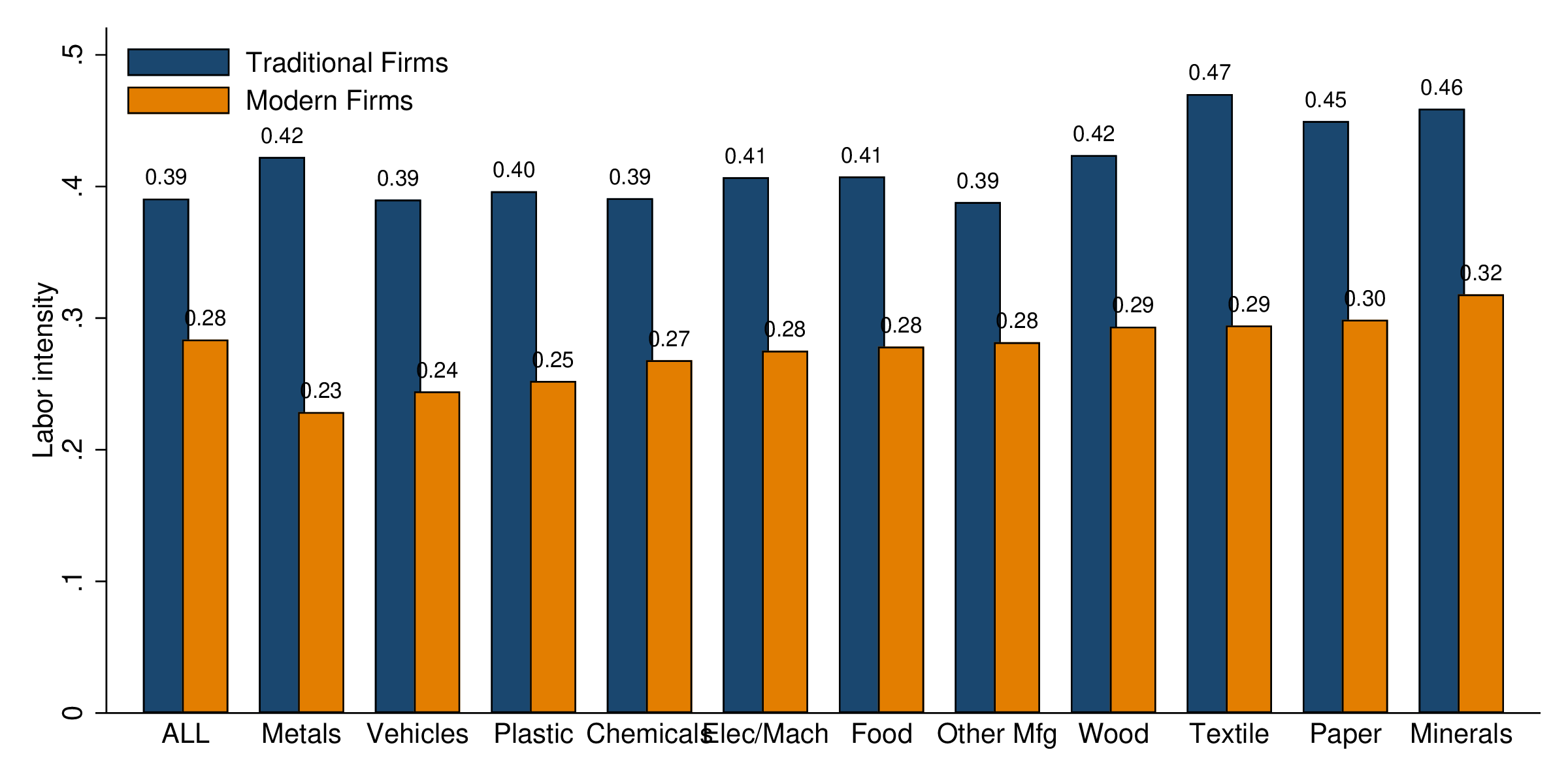 Notes: This figure shows our estimates of output elasticity of labor by firm status in terms of modern and traditional
technology, for the manufacturing industry as a whole, and by disaggregation, using firm-level data from WBES.
Section F provides details about the methodology that we apply to estimate production technologies and assign
firms into modern and traditional technological types.
Notes: This figure shows our estimates of output elasticity of labor by firm status in terms of modern and traditional
technology, for the manufacturing industry as a whole, and by disaggregation, using firm-level data from WBES.
Section F provides details about the methodology that we apply to estimate production technologies and assign
firms into modern and traditional technological types.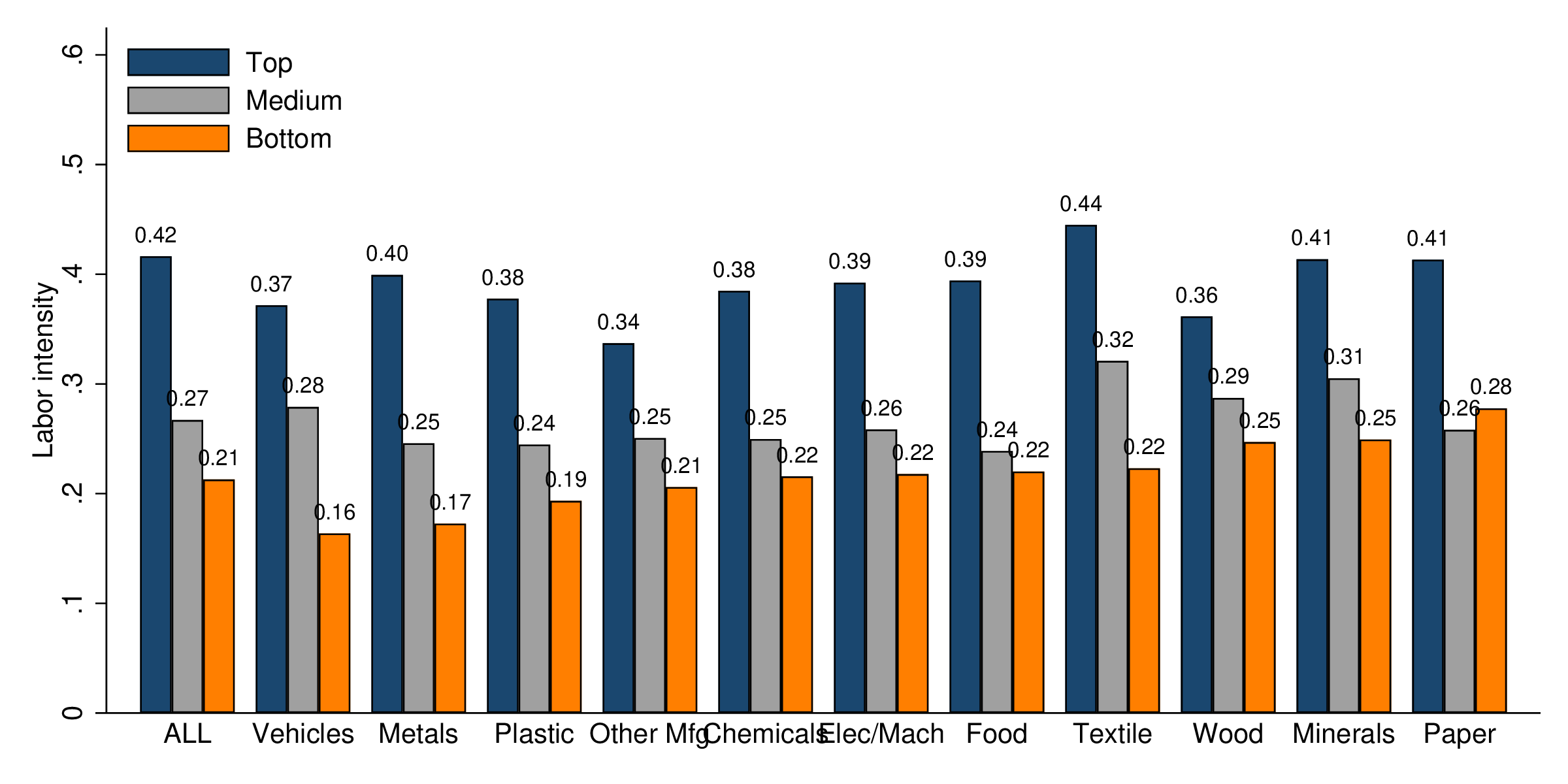 Notes: This figure replicates the exercise in Figure A.1 but using three technology regimes rather then two. Here, we
split the sample in terms of firm size according to three groups within each sector of the economy: (1) those in the
first quartile in the distribution of firm size; (2) those in the bottom quartile in that distribution; and (3) those in
the second and third quartile.
Notes: This figure replicates the exercise in Figure A.1 but using three technology regimes rather then two. Here, we
split the sample in terms of firm size according to three groups within each sector of the economy: (1) those in the
first quartile in the distribution of firm size; (2) those in the bottom quartile in that distribution; and (3) those in
the second and third quartile. Notes: This figure shows the distance to the efficient frontier (i.e., welfare costs of labor market distortions) for
closed economies. Quantifying the distance to the efficient frontier of closed economies requires two counterfactuals.
First, we move economies to autarky by raising trade costs to infinity. Second, in addition to moving economies to
autarky, we eliminate their labor market distortions. The difference between these two counterfactual outcomes
maps to the welfare cost of misallocation if countries were operating as closed economies. Each bar
shows our results by averaging them across countries in the high, middle, and low-income groups,
evaluated at three different values of the technology elasticity (\(\theta\)). The figure shows that the welfare cost of
misallocation is larger in low-income countries, and particularly more so when the technology elasticity (\(\theta\)) is
larger.
Notes: This figure shows the distance to the efficient frontier (i.e., welfare costs of labor market distortions) for
closed economies. Quantifying the distance to the efficient frontier of closed economies requires two counterfactuals.
First, we move economies to autarky by raising trade costs to infinity. Second, in addition to moving economies to
autarky, we eliminate their labor market distortions. The difference between these two counterfactual outcomes
maps to the welfare cost of misallocation if countries were operating as closed economies. Each bar
shows our results by averaging them across countries in the high, middle, and low-income groups,
evaluated at three different values of the technology elasticity (\(\theta\)). The figure shows that the welfare cost of
misallocation is larger in low-income countries, and particularly more so when the technology elasticity (\(\theta\)) is
larger. Notes: This figure shows the percentage change to real wage among low-income countries in response to a 20%
reduction in trade costs. The x-axis reports changes under the status quo labor wedges, the y-axis reports changes
under no labor wedges.
Notes: This figure shows the percentage change to real wage among low-income countries in response to a 20%
reduction in trade costs. The x-axis reports changes under the status quo labor wedges, the y-axis reports changes
under no labor wedges.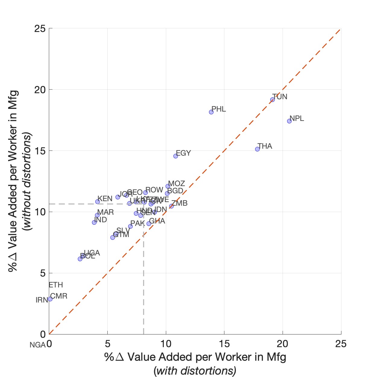 Notes: This figure shows the percentage change to value added per worker in manufacturing among low-income
countries in response to a 20% reduction in trade costs. The x-axis reports changes under the status quo labor
wedges, the y-axis reports changes under no labor wedges.
Notes: This figure shows the percentage change to value added per worker in manufacturing among low-income
countries in response to a 20% reduction in trade costs. The x-axis reports changes under the status quo labor
wedges, the y-axis reports changes under no labor wedges.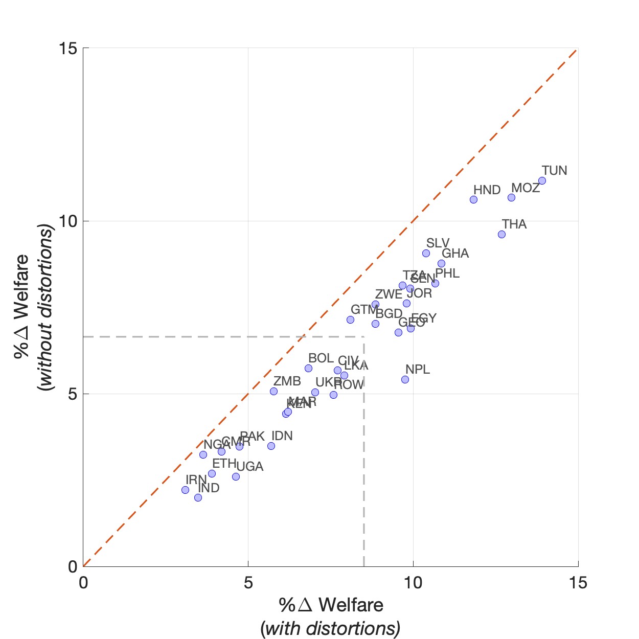 Notes: This figure shows the percentage change to aggregate welfare among low-income countries in response to a
20% reduction in trade costs. The x-axis reports changes under the status quo labor wedges, the y-axis reports
changes under no labor wedges.
Notes: This figure shows the percentage change to aggregate welfare among low-income countries in response to a
20% reduction in trade costs. The x-axis reports changes under the status quo labor wedges, the y-axis reports
changes under no labor wedges.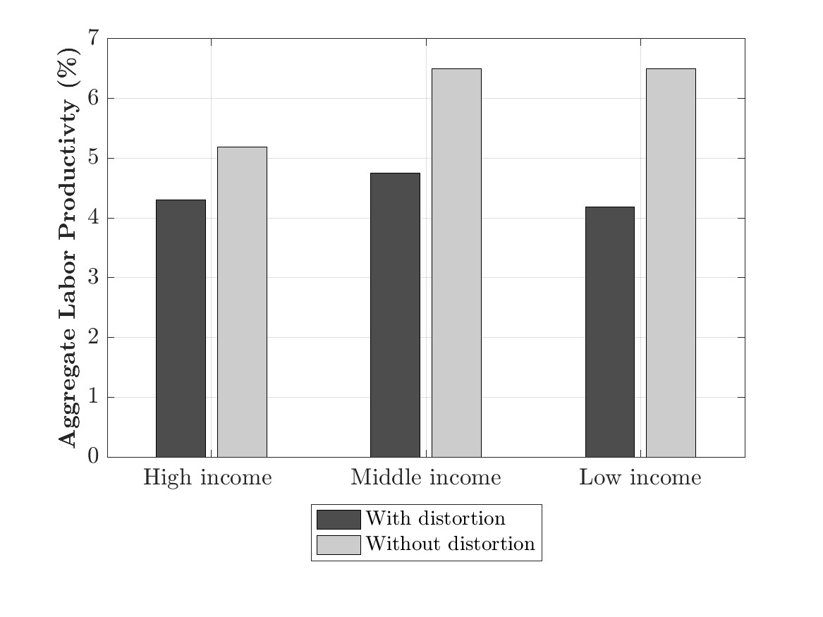 Notes: This figure shows the percentage change to aggregate labor productivity in response to a 20% reduction in
trade costs, averaging the results for low, middle, and high-income country groups.
Notes: This figure shows the percentage change to aggregate labor productivity in response to a 20% reduction in
trade costs, averaging the results for low, middle, and high-income country groups.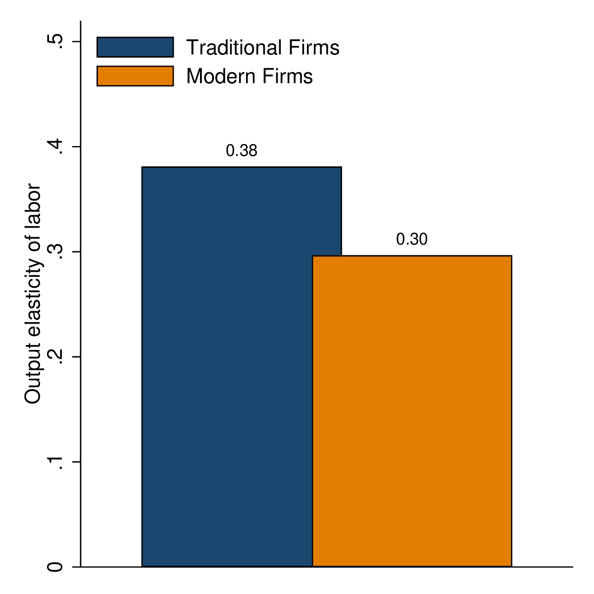
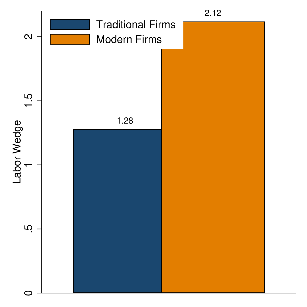
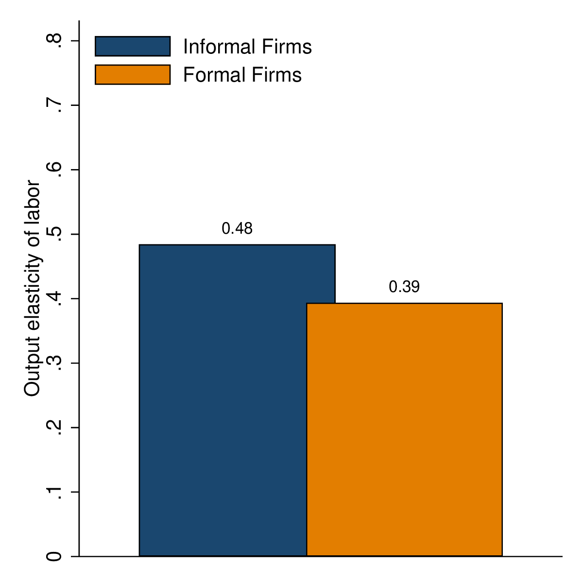
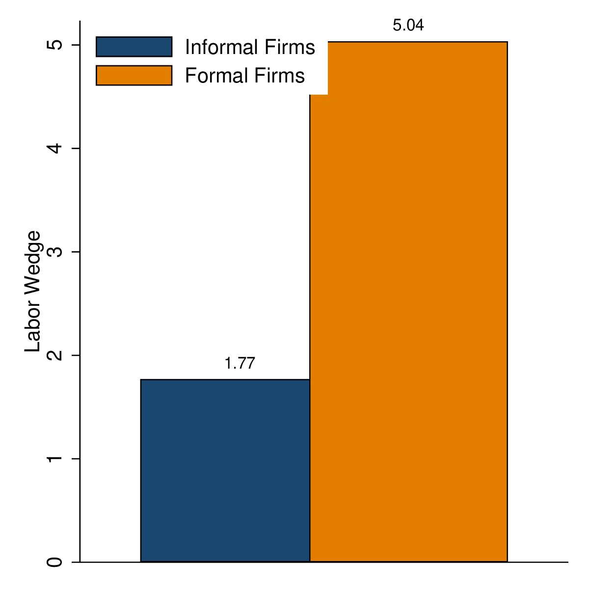
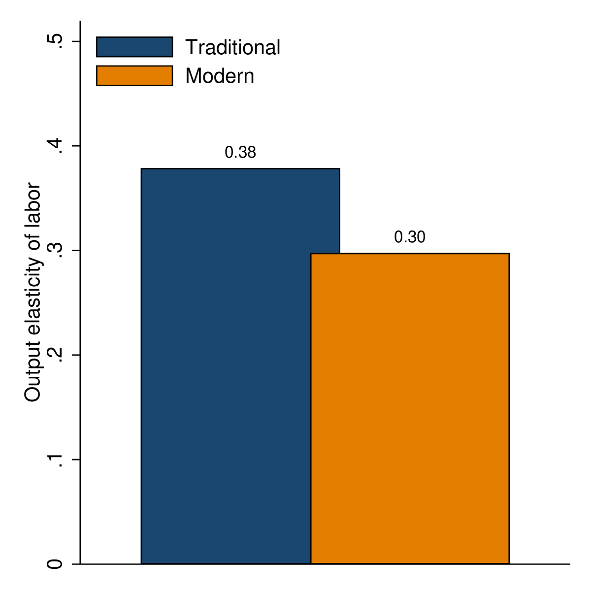
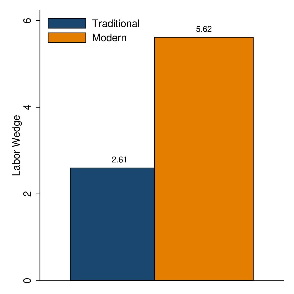
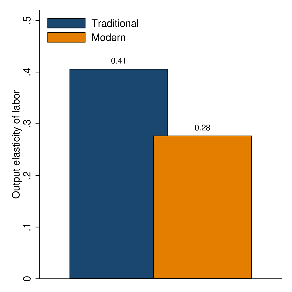
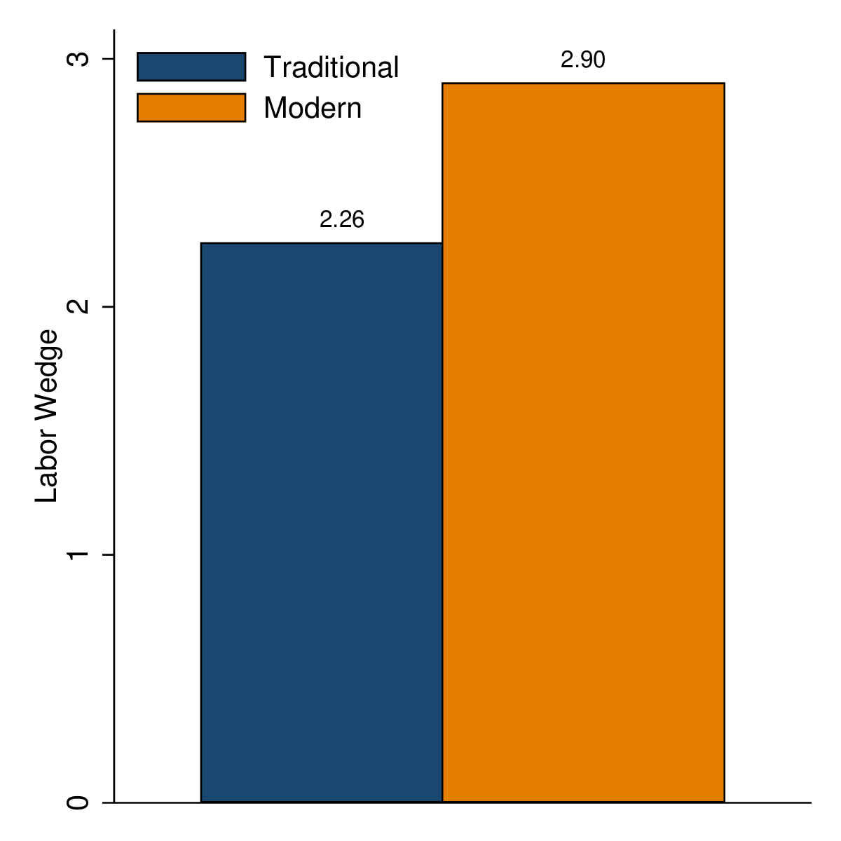
Multiple Technologies | Formal vs. Informal | ||
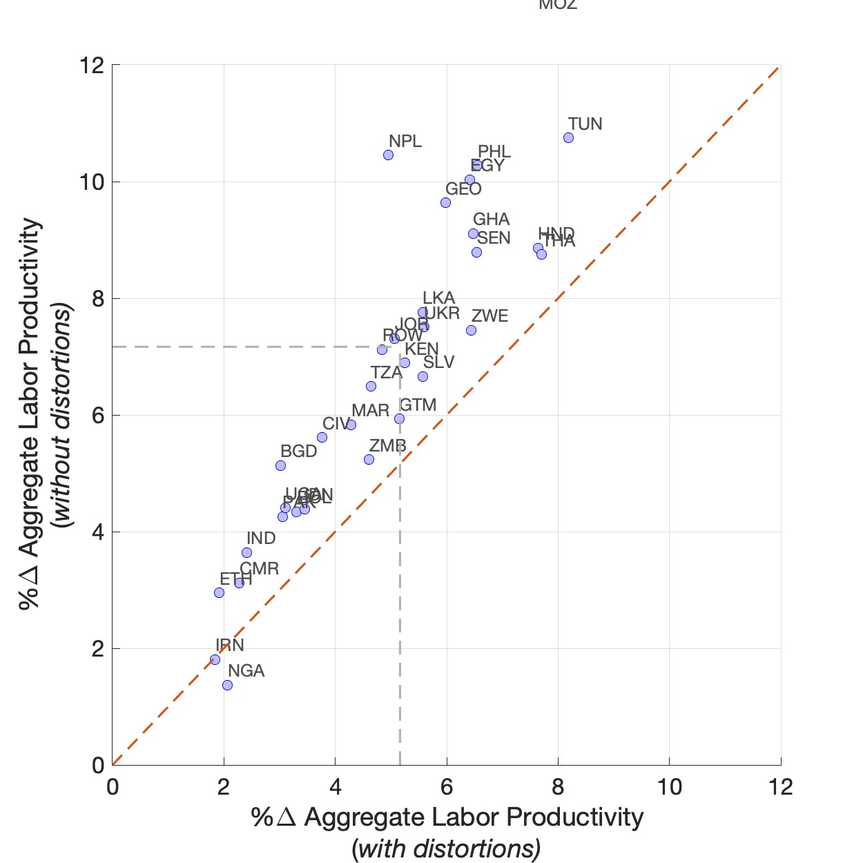 (a)
ALP (a)
ALP | 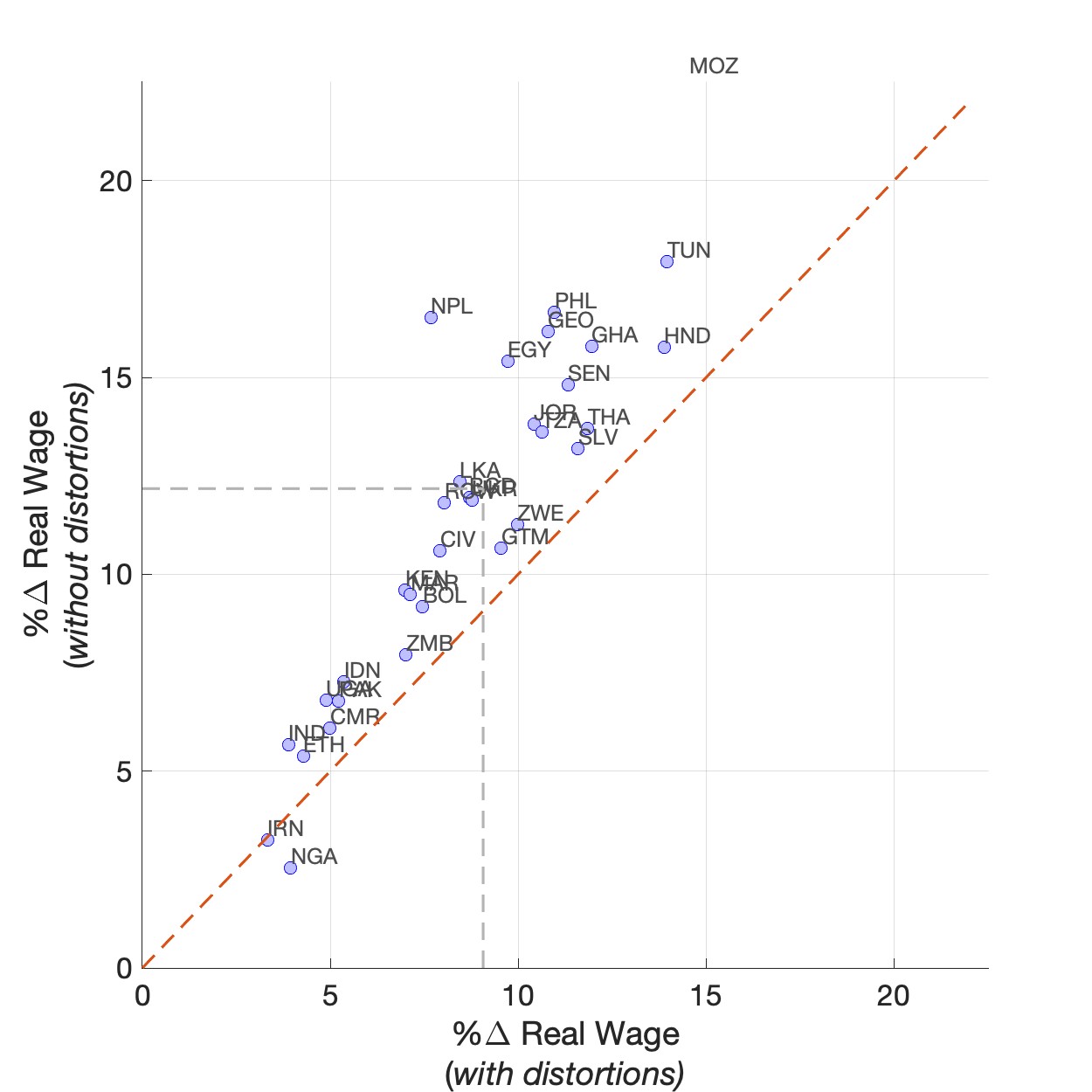 (b)
Real
Wage (b)
Real
Wage | 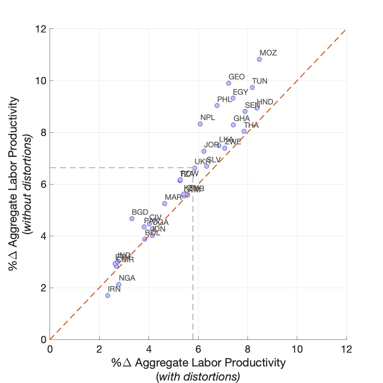 (c)
ALP (c)
ALP | 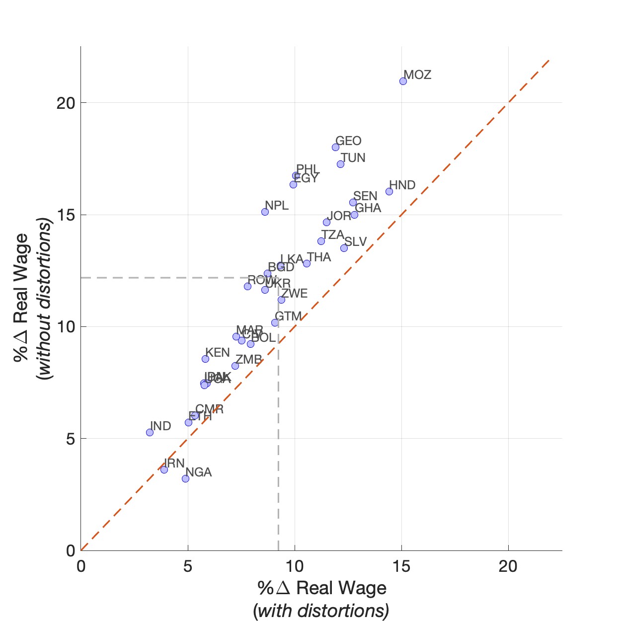 (d)
Real
Wage (d)
Real
Wage |
Low Theta | High-Theta | ||
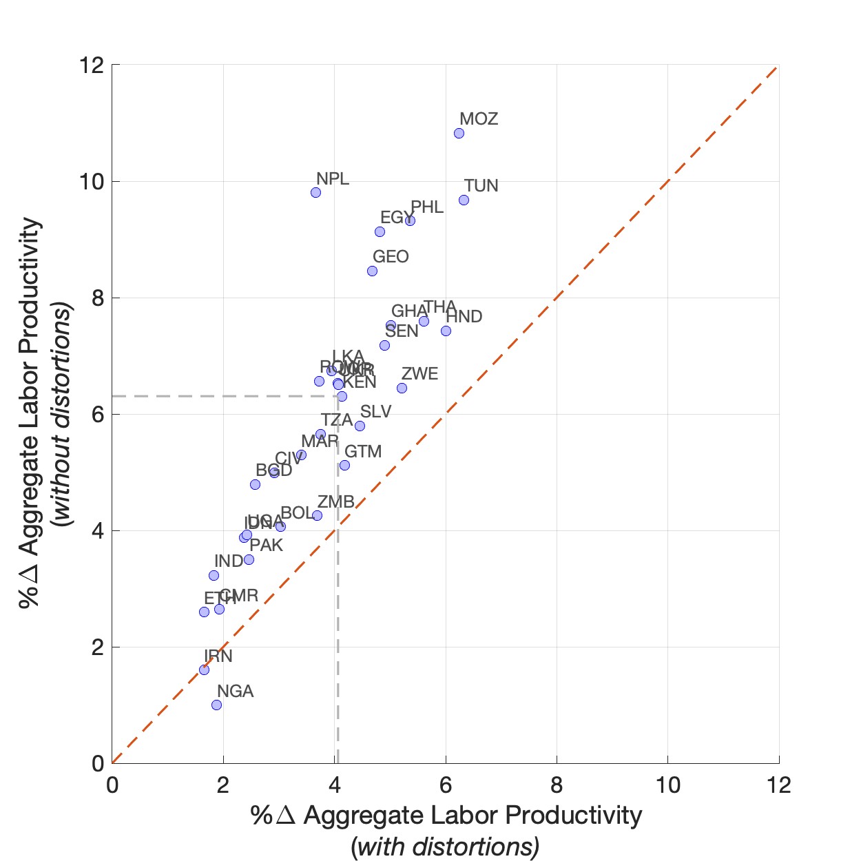 (e)
ALP (e)
ALP |  (f)
Real
Wage (f)
Real
Wage | 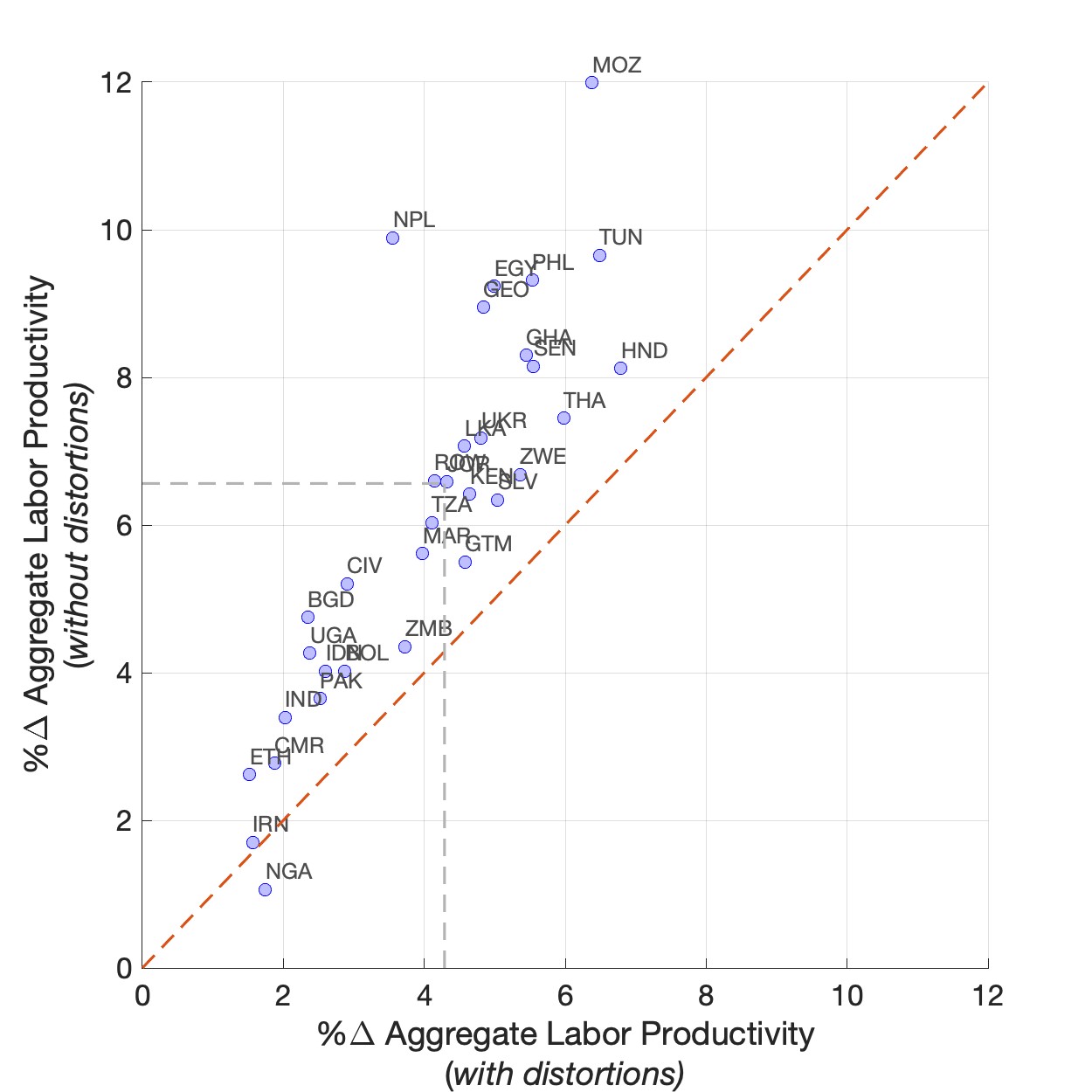 (g)
ALP (g)
ALP | 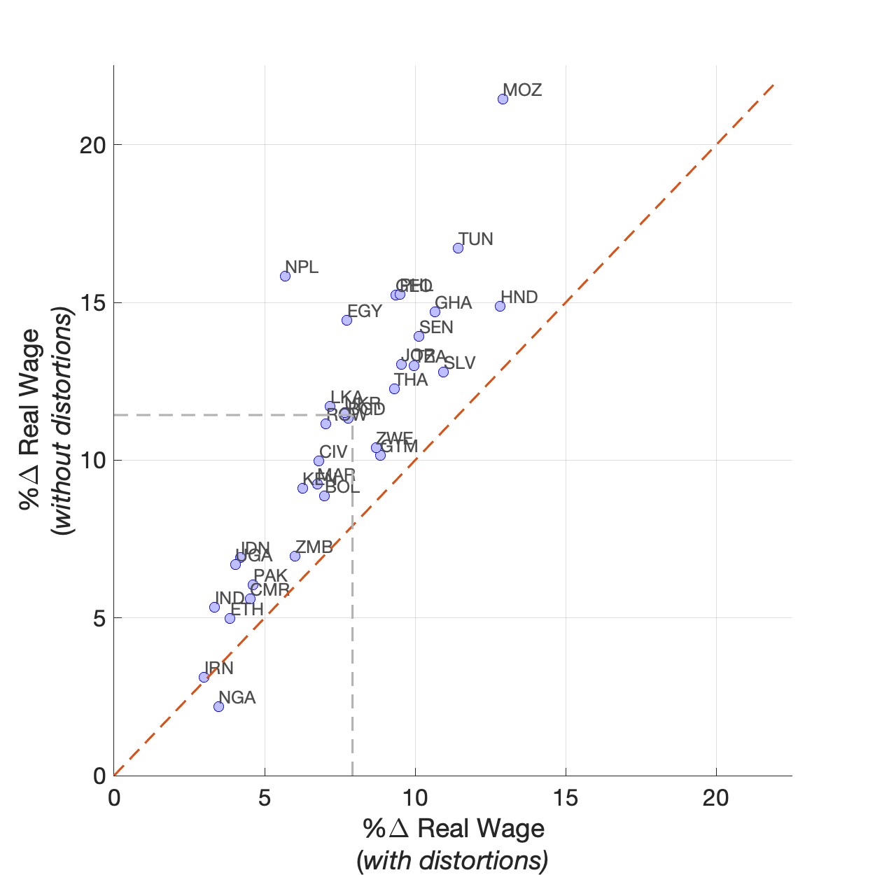 (h)
Real
Wage (h)
Real
Wage |
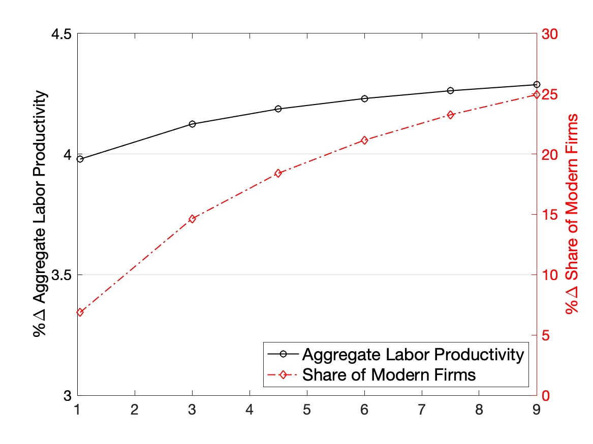 Notes: This figure shows, for each value of the technology elasticity (\(\theta\)) on the x-axis, the percentage change
(averaged across low income countries) to the share of modern firms (right-hand side y-axis) and aggregate labor
productivity (left-hand side y-axis) in response to a 20% reduction in trade costs.
Notes: This figure shows, for each value of the technology elasticity (\(\theta\)) on the x-axis, the percentage change
(averaged across low income countries) to the share of modern firms (right-hand side y-axis) and aggregate labor
productivity (left-hand side y-axis) in response to a 20% reduction in trade costs.